Introduction

Metastatic renal cancer (MRC) remains unlocated after a face-to-face examination and there are no primary tumour features in the kidney [1]. More than 60% of tumours are associated with malignant metastases after the first consultation, of which approximately 10% metastasise to the patient’s kidney [2]. MRC accounts for 1% to 1.5% of all malignant clinical cases [3], ranking 13^th in malignancy [4] and 7^th in mortality and recurrence rates [5]. Afrit et al. reported that the average survival time of patients with MRC after multiple consultations was 3.8 months, with a 1-year survival rate of 18.7%; 5-year survival rate of 4.1% and 10-year survival rate of 2.8%. The authors concluded that prognostic status was governed by the tumour’s domination by the biology of the primary tissue [6]. Metastasectomy and/or targeted therapies may play role in prolonging short-term survival rates but unfortunately cannot ensure a complete cure from metastatic cancer [7, 8]. Therefore, tracing the tissue origin of MRC is crucial for physicians to design treatment plans, enabling precise treatment and improving patient prognosis.

Metastatic kidney cancer is histologically heterogeneous and physicians are unable to improve the pathological mechanism of the tumour, which often leads to misdiagnosis and underdiagnosis. Immunohistochemistry is not only used as a concomitant immunosuppressant in steroid-dependent nephrotic syndrome [9] but is also the most commonly used clinical method to locate the primary tumour and can provide a practical reference for physicians in diagnosis and treatment [10]. However, at present, immunohistochemistry methods rely on small sample data, are labour-intensive, have moderate classification accuracy, and have high breakthrough costs, which need to be improved [11]. Computed tomography (CT) and positron emission tomography (PET) can be used to identify the origin of cancer tissue using medical imaging techniques with relative ease and speed, but with an accuracy of only 20–27% and 24–40%, the performance needs to be improved [12]. Therefore, the development of a new, efficient and convenient method to probe the pathological origin of cancer appears urgent and necessary in clinical applications.

A related study reported that metastatic cancer foci could not replicate the structural features of the primary tumour but could still carry the gene expression profile of the original tissue. Lu et al. screened 80 differentially expressed genes (DEGs) by raw signal analysis and constructed three medical prediction models – random forest (RF), support vector machine (SVM) and neural network – then used them to distinguish four types of squamous cell carcinoma to trace the tissue origin of metastatic cervical cancer [13]. By analysing gene expression profiles, Wang et al. constructed a database containing 96 specific genes; the database was screened for key genetic information to produce molecular markers, followed by inference of the tissue origin of 22 common metastatic malignancies [14]. Zhao et al. trained a one-dimensional convolutional neural network medical prediction model to classify the primary tumour database to locate the tissue origin of unknown primary carcinoma (CUP) by constructing a one-dimensional convolutional neural network [15]. It is evident that the use of machine learning methods to construct medical tracing models and map gene expression profiles to infer the tissue principles of malignant tumours has become a popular aid to diagnosis and treatment. The incidence of metastasis to the kidney varies among different sites of malignancy, with lung adenocarcinoma, lung squamous cell carcinoma, liver hepatocellular carcinoma and pancreatic adenocarcinoma having a total metastasis rate of 45–65% and being the main malignant origin of MRC [16]. Therefore, the study will analyse data on gene expression of primary and MRCs from a bioinformatics perspective and construct five machine learning models to pinpoint the malignant origin of cancer.

Material and methods

Traditional modelling methods

SVM model

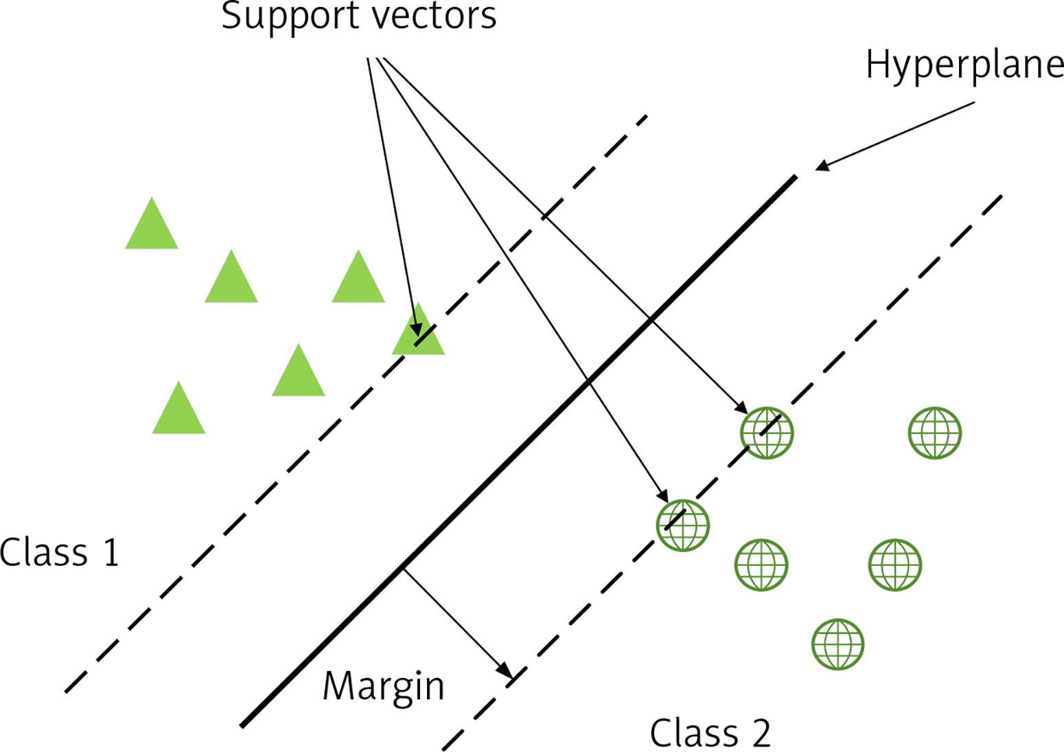
An SVM is a binary classification model whose basic model is a linear classifier defined by maximising the interval on the feature space, which distinguishes it from a perceptron; SVMs also include kernel tricks, which make them essentially non-linear classifiers. The learning algorithm for SVM is the optimisation algorithm for solving convex quadratic programming. As in Figure 1, support vectors (SV) are used to limit the width of the model edges. The core idea of the SVM is to divide the input fields into 2 sets of vectors in a multidimensional space and construct a hyperplane to separate the input vectors, which maximizes the boundary between the 2 sets of input vectors [17].

Figure 1

SVM schematic diagram

Decision tree (DT) model

A DT is a model that presents decision rules and classification results in a tree-like data structure. As an inductive learning algorithm, the focus is on taking seemingly disordered and disorganised known data and transforming them by some technical means into a tree model that can predict unknown data. Each path in the tree from the root node (the attribute that contributes most to the final classification result) to a leaf node (the final classification result) represents a rule for making a decision. The DT diagram (Figure 2) is as follows [18, 19].

Figure 2

DT schematic diagram

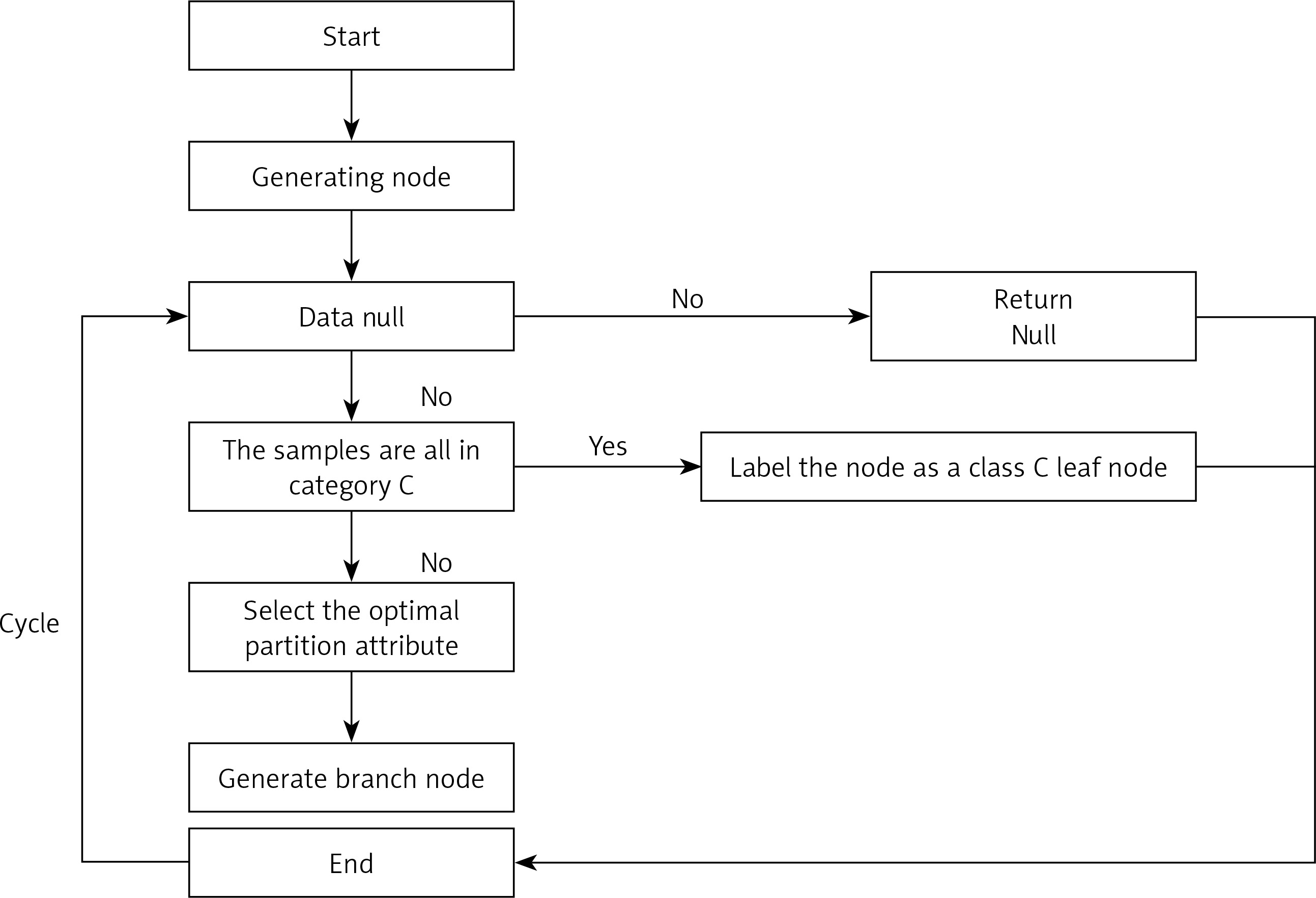
1. Firstly, from the start position, divide all the data into one node, the root node.

2. Then go through the two steps in orange, with the orange indicating the judgement condition.

3. If the data are the empty set, jump out of the loop. If the node is the root node, return null; if the node is an intermediate node, mark the node as the class with the most classes in the training data.

4. If the samples all belong to the same class, skip the loop and the node is marked as that class.

5. If none of the judgment conditions marked in orange jump out of the loop, the node is considered for division. Since this is an algorithm, the division should not be done arbitrarily, but with efficiency and accuracy, choosing the best attribute division under the current conditions.

6. After going through the division in the previous step, a new node is generated, and then the judgment condition is cycled, and new branching nodes are continuously generated until all nodes have jumped out of the loop.

7. End. This results in a DT.

RF model

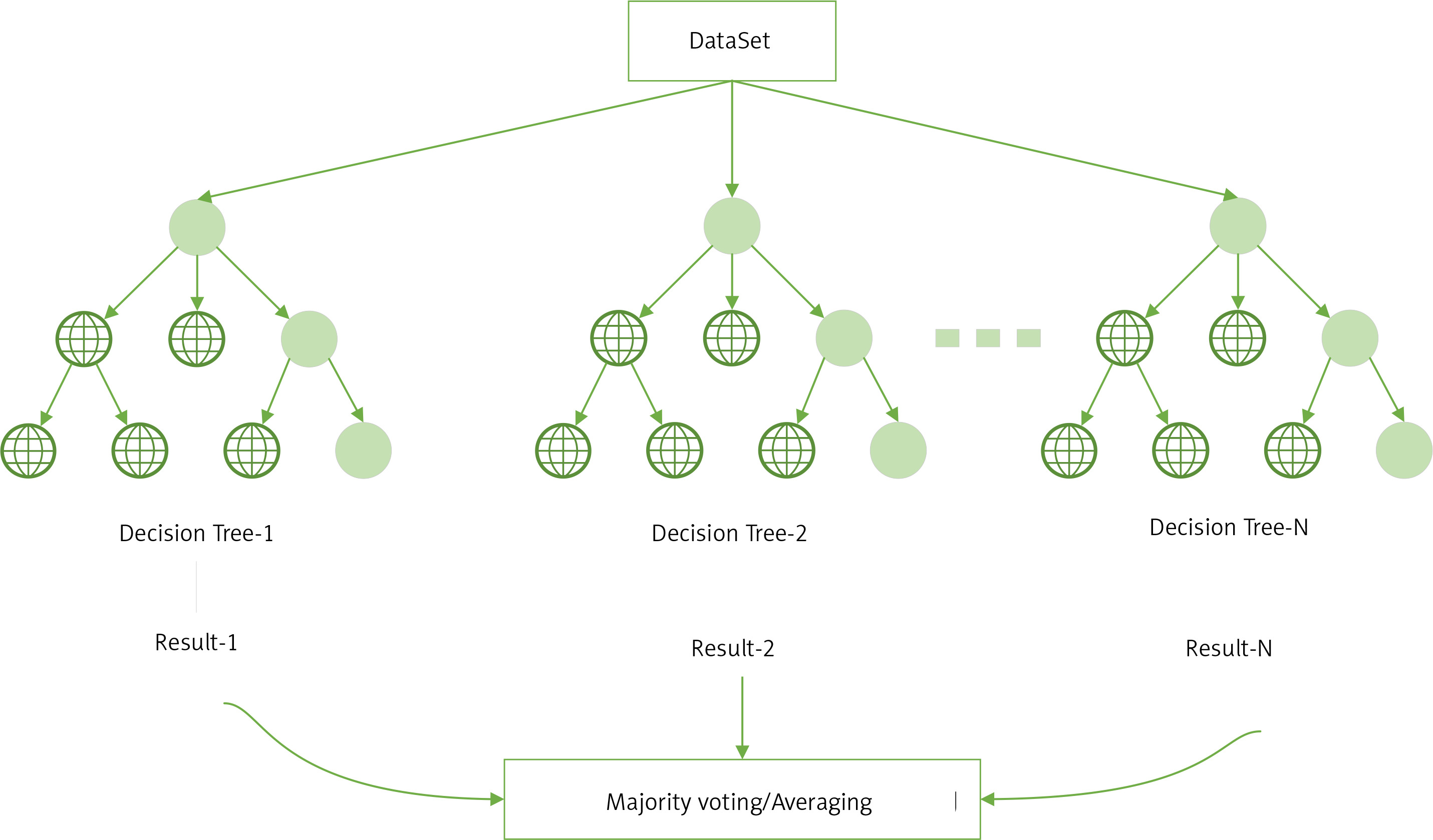
RF is an ensemble learning algorithm of the bagging type, which combines multiple weak classifiers (DTs) and the final result is obtained by voting or taking the mean, making the overall model result highly accurate and generalisable, as shown in the structure below (Figure 3) [20]. Its good results can be attributed to ‘random’, which allows it to resist over-fitting, and ‘forest’, which makes it more accurate [21].

Figure 3

RF structure

Improved RF modelling approach

Improved Relief (ReliefFk) algorithm

The binary filtered feature selection (Relief) algorithm can be used to solve the feature weight calculation in binary classification problems. ReliefF is an optimisation of Relief that can be used in multi-classification scenarios [22]. In this section, the ReliefF algorithm is incorporated into the feature selection step of the RF construction DT, which can initially remove some of the features that negatively affect the model, and can also be used to alleviate the problem of false high or low classification accuracy caused by imbalance in medical data.

The core idea of the Relief algorithm is to use the correlation between positive (1) and negative classes (0) and features as a reference basis for assigning specific weights to each feature attribute. The basic idea is that the feature is preferred, a random sample is selected from the test set, the most similar sample of the same type (same spe) and the most similar sample of the different class (diff spe) are selected, and the mean distance between the feature and the same spe and diff spe samples is calculated successively. If there is a difference in the mean distance between the two classes, it means that the feature has a strong ability to differentiate between the samples of the current class. Conversely, if the mean distance values are the same or similar, it means that the distinguishing ability needs to be improved, and the weight of the feature should be reduced. The formula for calculating the weights can be expressed as [22, 23]:

(1)

W(a)=W(a)−diff(a,r,s)m+diff(a,r,d)m,

where W (a) is the feature a weight.

The ReliefF algorithm is a modification of the Relief algorithm, based on which a multi-categorisation strategy is added. The basic idea is that instead of taking positive and negative samples, a sample is taken from each category and the weights of the features are calculated and updated. This not only solves the multi-category problem, but also indirectly reduces external noise interference and improves the stability of the algorithm. The weighting formula is updated to [22]:

(2)

W(a)=W(a)−∑j=1kdiff(a,r,Hj)mk++∑C∉class(r)[p(C)1−p(class(r))∑j=1kdiff(a,r,Mj(C))]mk,

p(C) is the proportion of class C samples in the original data, Mj(C) is the j nearest neighbour sample in class C ∉ class(r), and diff(a, r₁, r₂) represents the difference in distance between samples r₁ and r₂ on feature a, which can be expressed as [23]:

(3)

diff(a,r1,r2)={|r1[a]−r2[a]max(a)−min(a),if a is continues0, if a is discrete and r1[a]=r2[a]1, if a is discrete and r1[a]≠r2[a],

From Equation (3), the ReliefF algorithm averages the distance differences between the k samples closest to x_i in heterogeneous class C on feature a and multiplies this by the proportion of heterogeneous class C samples to all heterogeneous samples from x_i. This operation is repeated for all heterogeneous samples from x_i, resulting in the mean value of the distance differences between samples in heterogeneous class C on feature a. W = {w₁, w₂, w₃,…, w_n} is the weight vector obtained by the ReliefF algorithm, and the features are sorted in reverse order by weight value.

The improved idea of the ReliefF algorithm is for the multi-category problem. The algorithm uses random function for random sampling among different categories of samples, which can achieve a better anti-noise interference effect and maintain certain stability under normal circumstances. In practice, however, the mean distance between heterogeneous samples and features a is large, and the mean distance between similar samples and features a is small; therefore, it is mainly the heterogeneous sample values that open up the weight gap (mean distance difference) and guarantee the stability of the weight gap. Therefore it is also necessary to slightly improve the sampling steps of the algorithm to obtain the ReliefFk algorithm: reduce the sampling weight of similar samples, increase the sampling weight of each class of heterogeneous samples, stabilize and refine the distance mean between heterogeneous samples and feature a, in order to allow a variety of heterogeneous samples with high decision power. The specific implementation steps are: Assume that n is the number of samples in the medical training set, where the number of positive class samples is n₊ and the number of negative class samples is n_. Let the initial number of nearest neighbour samples in the training set be k, the number of nearest neighbour like samples be k₁, the number of nearest neighbour dissimilar samples be k₂ and the initial k₁ = k, k₂ = k. If sample r is a positive class, then k₁ and k₂ can be expressed as:

(4)

k1=k*n+n++n−,

(5)

k2=kn++n−n−,

When the sample taken r is a negative class, k₁ and k₂ can be expressed as

(6)

k1=k*n−n++n−

(7)

k2=kn++n−n−,

When calculating the weights of the characteristics a, the number of samples of the two categories of similarity and dissimilarity is changed from k to k₁ and k₂ respectively, and k₁ < k, k₂ > k; this theoretically reduces the proportion of samples of similarity and increases the proportion of samples of dissimilarity in each category, giving more decision power to the dissimilar samples and guaranteeing the stability of the distance difference (characteristic weights). The improved weighting formula is as follows.

(8)

W(a)=W(a)−∑j=1k1diff(a,r,Hj)mk1++∑C∉class(r)[p(C)1−p(class(r))∑j=1k2diff(a,r,Mj(C))]mk2,

Heterogeneous filtered feature selection random forest (ReliefFk_RF) algorithm

As shown in Figure 4, the ReliefFk algorithm is incorporated into the RF algorithm to form the new algorithm ReliefFk_RF algorithm: firstly, the formula for calculating the weights of the ReliefF algorithm is modified (reducing the sampling weight of similar samples k₁ and increasing the sampling weight of each class of dissimilar samples k₂), then some of the attribute features that have no effect on the classification results are initially screened out, and the remaining attribute features are ranked by their weights, and the training subset of the attributes of the training subset are divided equally into three intervals of high, medium and low weights. When RF enters the DT construction step, a subset of features with uniform classification effect is used to train the DT, and the set of features in the three intervals is drawn evenly, which can effectively avoid too many redundant features being repeatedly drawn, reduce the trouble of poor classification performance and enhance DT stability.

Figure 4

Flowchart of ReliefFk algorithm integrated into RF algorithm

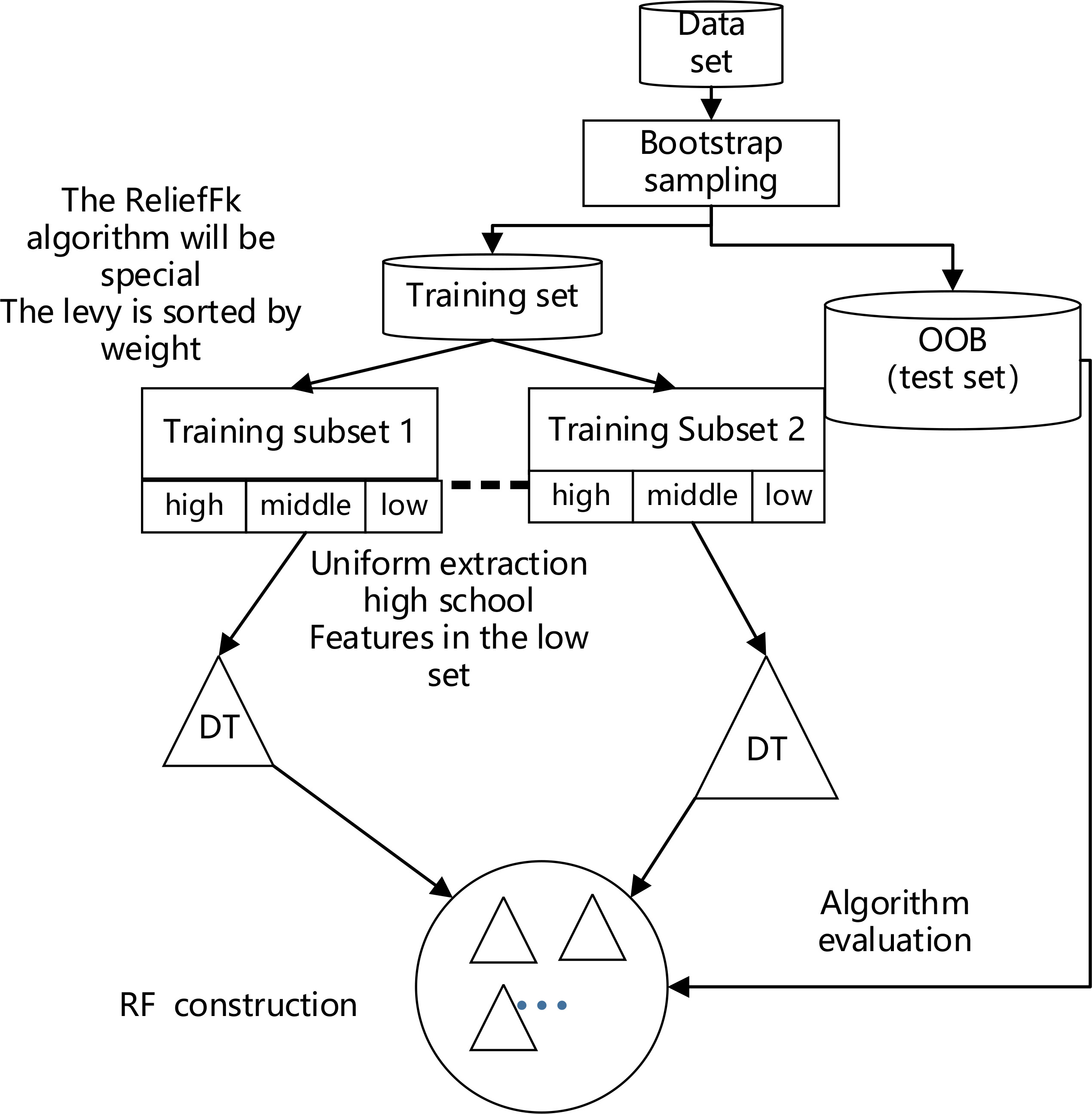
As shown in Figure 4 above, the model performs bootstrap sampling of the dataset to obtain various training subsets and OOB test sets (the out-of-bag dataset can be used for final model evaluation); the extracted dataset is then sorted by the weights of the ReliefFk features to obtain the set of features with the attribute weights. The larger the weights of the features, the higher is the classification performance. The sorted attribute features are divided into three classes (high, medium and low) according to their classification performance. When the DT is constructed, the traditional form of random sampling is discarded and the features are drawn equally in the set of three classes to evenly consider the classification performance of each class of attributes and indirectly guarantee DT stability. The DT is constructed by continuously extracting features in sequence for multiple training subsets to form the final RF, and the algorithm1 pseudo-code is as follows (Algorithm 1).

The aim of the ReliefFk_RF algorithm is to modify the formula for calculating the weights of the ReliefF algorithm to remove the features that are not useful for the overall classification effect; then the remaining features are evenly differentiated according to their weights, so that the features in each weight range can be evenly sampled during DT construction, effectively avoiding too many redundant features being repeatedly selected, and also indirectly alleviating the problem of false high or false low classification accuracy, and stabilizing the DT accuracy.

Algorithm1: ReliefFk_RF Core steps pseudo-code

Input: Training set D;

  Sampling frequency m, initial m = 10;

  Characteristic dimension n, feature weight set W_i

  Initially null;

  k, k₁, k₂ are the number of nearest neighbour

  samples drawn from each of the D categories.

Output: Set of highly differentiated features W_h;

  Feature set of medium distinction W_m;

  Low distinction feature set W_l.

1. Set all feature weights W_i. = 0, i = 1,2,…,n to 0;

2. for i = 1 to m do

   1. A single sample is randomly selected from D set r;

   2. Find k₁ nearest neighbour Hj(j = 1,2,…,k) samples from the similar sample set of r, k₂ nearest neighbour Mj(C) samples are found from the heterogeneous sample set of r;

   3. for a = 1 to n (all features) do Updating feature weights with ReliefF algorithm:

      W(a)=W(a)−∑j=1k1diff(a,r,Hj)mk1++∑C∉class(r)[p(C)1−p(class(r))∑j=1k2diff(a,r,Mj(C))]mk2

   4. end;

3. end;

4. Delete the feature with a weight of 0;

5. W_h = W_i, i = 1,2,…, n/3;

  W_m = W_i, i = n/3 + 1,…, 2n/3;

  W_l = W_i, i = 2n/3,…, n;

Heterogeneous filtered feature selection random forest weighted (ReliefFk_RFw) algorithm

The traditional RF assumes equal weights for each DT, ignoring the variability among DTs. Based on this, this paper proposes a DT error weighting of the previous ReliefFk_RF algorithm to obtain the ReliefFk_RFw algorithm, with the weighting formula for a single DT as [24]:

(9)

W(i)=1/|2(i)∑j=1T1/|2(j),

where w(i) is the weight of the i-th DT and I²(i) is the variance of the difference between the predicted and actual points in the training set of the i-th DT. A larger value of I²(i) represents a lower stability of DT prediction, so the weight is smaller. The DT weighting parameters proposed in the study satisfy the normalisation feature [24].

(10)

∑i=1Tw(i)=∑i=1T(1/|2(i)∑j=1T1/|2(j))=∑i=1T1/|2(i)∑j=1T1/|2(j)=1,

The ReliefFk_RFw algorithm regression algorithm process is:

1. Generate multiple stable DTs using the ReliefFk_RF algorithm.

2. When training the i-th DT, the distance variance I²(i) between all predicted and actual points in the DT is calculated and the weight values are obtained as:

   (11)

   w(i)=1/|2(i)∑j=1T1/|2(j),

3. The weighted predicted value û(x) of the ReliefFk_RFw algorithm is expressed as:

   (12)

   u^(x)=∑i=1Tw(i)Yi,

Where Y_i is the initial predicted value of the i-th tree DT.

Results

Characteristic gene selection

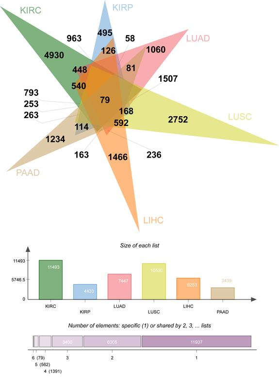
At the initial stage of the study, there were 69,672 genes, which was of low representativeness. The T. est function was used to calculate the difference between each gene in primary tissue (group1=case) and normal control tissue (group2=control not determined). After that, the p.adjust function was called to calculate the fixed significance FDR of each gene and evaluate the differences of each gene. The Venn diagram (Figure 5) shows the DEG data relationship among six types of cancer. KIRC, KIRP, LUAD, LUSC, LIHC and PAAD contain 11493, 4433, 7447, 10530, 6253 and 3439 DEGs respectively. A total of 4930 (KIRC), 495 (KIRP), 1060 (LUAD), 2752 (LUSC), 1466 (LIHC), and 1234 (PAAD) “specific” DEGs were included in the differential expression information (only significantly expressed in one malignancy, Figure 5).

Figure 5

Venn diagram of DEGs

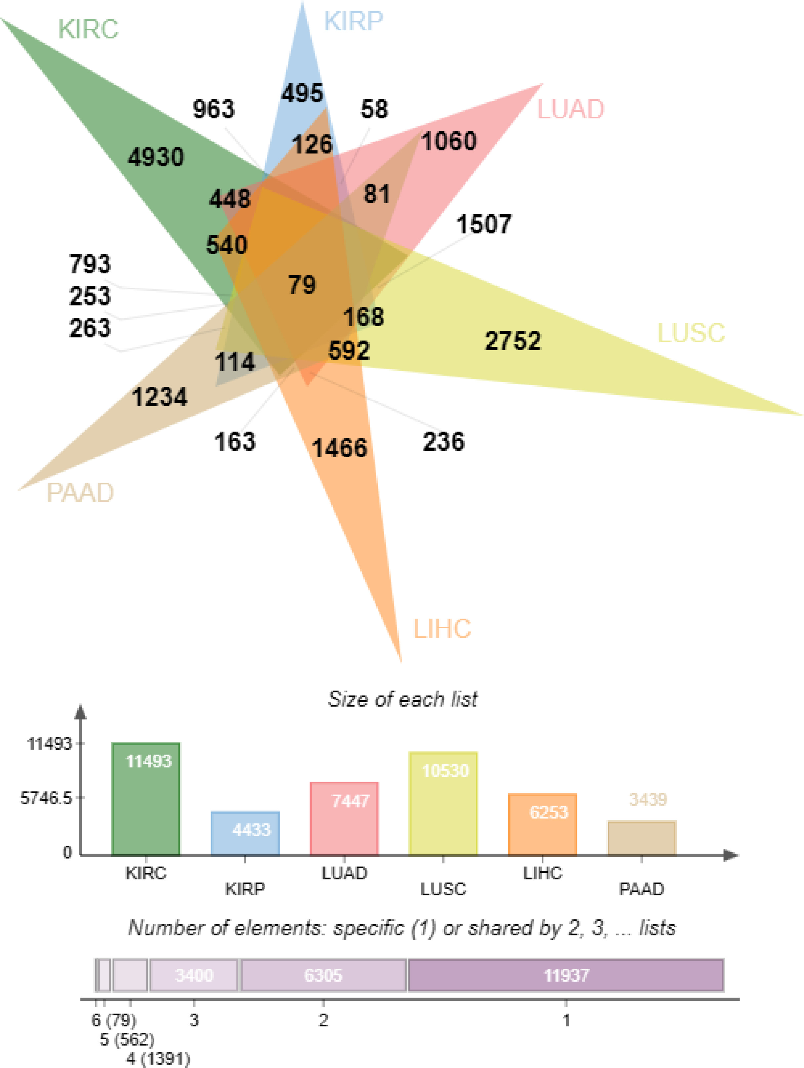
The “specific” DEGs in the top 5% of cancer differential expression values were extracted (247 KIRC, 25 KIRP, 53 LUAD, 138 LUSC, 74 LIHC and 62 PAAD, for a total of 599 “specific (the “DEGs”). The genetic information following signature gene selection was genetic data for significant differences between each primary cancer and conventional controls, and the ‘signature’ DEGs were mutually exclusive between cancer types.

Discussion

In this study, the ReliefFk_RFw model was created by rewriting the pseudo-code at the bottom of the algorithm, and the effects of the primary tissue of MRC were compared with the SVM, DT and RF models. The ReliefFk_RFw model has the best overall evaluation results, which effectively verifies the existing hypothesis that “metastatic tissue retains genetic characteristics of origin”, and can assist in guiding clinical diagnosis and treatment. Faced with diagnosis of MRC, physicians can create an improved ReliefFk_RFw model, input patient-specific “DEGs” in order of importance, and evaluate the output by classification to locate the primary origin of metastatic tissue. Assuming that the output was cancerType=4 (primary origin =LUSC), the physician recommended a combination treatment regimen dominated by lung squamous cell carcinoma and assisted by kidney cancer, and was on high alert for re-metastasis of tissue origin during follow-up. The clinical treatment plan and follow-up plan are developed according to the specific disease occurrence of patients and doctors’ experience. The output results of this study model are only for auxiliary reference.

This study combined machine learning and differential expression analysis techniques to initially screen out “specific” DEGs to reduce the model prediction dimension, increase the data relevance, and effectively improve the accuracy of tracing results. Although the traditional machine learning model can carry out feature screening, its understanding of bioinformatics information is only at the data level, unable to analyse the correlation of genetic data, so the traceability performance is limited. Differential expression analysis could select 599 “specific” DEGs with significant expression from 69,672 genetic genes of the initial malignant tumour according to the up-down-regulated gene scores of fixed cancer. Selected “specific” DEGs can control the physiological mechanism and biological development form of cancer, and are the main driving force for regulating the life activity process of cancer cells [30]. At the initial stage of the study, differential expression analysis can effectively distinguish the biological differences between different primary cancers and surrounding conventional tissues; at the middle stage, the machine learning algorithm can distinguish the genetic differences between different primary cancers; at the later stage, the improved ReliefFk_RFw model can achieve a leapfrog improvement in the precision of the primary tissue trace procedure. Therefore, in feature engineering, differential expression analysis is adopted to screen “specific” DEGs, which can fill the gap in the biology of machine learning algorithms and provide an experimental reference for machine learning engineers.

In this study, five evaluation indexes (accuracy, precision, sensitivity, specificity and F1 Score) were used to comprehensively measure the multi-category classification ability of the machine learning model. The average accuracy, precision, sensitivity, specificity and F1 Score of the ReliefFk_RFw model are as high as 98.89%, 99.90%, 99.11%, 99.53% and 99.36%, and the retrospective effect is even better than that of the popular medical aid methods of image parsing and deep learning in recent years. For example, Jin et al. developed a deep learning system based on preoperative CT images of gastric cancer patients, which was used to predict lymph node metastases of multiple lymph nodes. The results of image analysis showed excellent prediction accuracy in the external validation queue, but the sensitivity (0.743) and specificity (0.936) were still lower than 0.989 and 0.999 of the ReliefFk_RFw model in this study [31]. Doppalapudi et al. performed a feature-importance analysis to understand how factors related to lung cancer affected survival in patients. The classification accuracy of the recurrent neural network (RNN) model in the deep learning field is 71.18%, lower than the 99.53% of the ReliefFk_RFw model in this study [32]. Liu et al. explored the value of deep learning (DL) based on global digital mammography in the prediction of microcalcification malignancy in the Breast Imaging Reporting and Data System (BI-RADS) 4. The combined DL model showed good sensitivity and specificity of 85.3% and 91.9%, respectively, when predicting the four types of malignant microcalcifications of BI-RADS in the test data set, but these values were still lower than the 98.9% and 99.9% of the ReliefFk_RFw model in this study [33].

In diagnosis and treatment, mature medical instruments are often used to determine the origin of tissues. Although machine learning methods have begun to be used for primary tracing, precise localization of specific cancers has not yet been studied. This study proposed for the first time that the improved ReliefFk_RFw model could be used to predict the origin of MRC tissue, accurately match the specific “DEGs” and fix the genetic relationship between the primary cancer, and assist physicians in diagnosis and treatment, which has considerable medical significance. At present, clinical practices mostly use immunohistochemical methods to lock specific antigens (such as proteins, peptides, enzymes, etc.) and colour primary sites to assist in tracing the origin [34]. Although suitable immunoenzymatic techniques have been developed to establish a high degree of sensitivity with the primary tissue, they are still only suitable for small-scale data analysis and are labour-intensive, making it difficult to overcome the accuracy bottleneck [11]. CT and PET are the most convenient and rapid primary tissue tracing techniques at the present stage; they are powerful tools in medical imaging and can effectively distinguish benign and malignant tissues, but their low accuracy rates of 20–27% and 24–40% need to be improved [12]. Therefore, a new machine learning model tracing technology is needed to replace such low-accuracy, labour-intensive and data-dependent traditional detection technology. Tian et al. used RF and SVM models to screen biomarkers, and used minimum absolute contraction and selection operator (LASSO) regression analysis to construct multi-gene signatures. Univariate and multivariate Cox regression analysis was used to explore the relationship between clinical features and prognosis, which promoted the personalized management of patients with kidney cancer, showing advantages such as high accuracy, convenience, universality, non-invasiveness and repeatability [35]. It can be seen that the participation of machine learning models in the diagnosis and treatment of kidney cancer is convenient, accurate and efficient, and can effectively guide medical decision-making and assist diagnosis and treatment.

Although the improved ReliefFk_RFw model can effectively trace the origin of MRC, there are still some limitations in experimental studies. (1) Due to the lack of conventional tissue sample data of osteosarcoma in the TCGA database, there are only 6 cancerType values predicted by the model (KIRC, KIRP, LUAD, LUSC, LIHC, PAAD). (2) The study was limited to the organ-specific origin of MRC and did not consider the aggregation of origin outside the organ. For example, a study of unsupervised analysis of TCGA multi-genomic data suggested that primary malignant tissue may aggregate outside the organ of origin, or between unrelated organs, or as a heterogeneous tissue independent of existing medical tumour types [36].(3) In addition, only internal cross-validation was used in this study. Although the repeatability of the ReliefFk_RFw model was verified, the portability and generalization of ReliefFk_RFw need to be verified. Future research will adopt internal and external verification methods. On the basis of ensuring model stability (internal verification), external verification such as spatial verification, time period verification and domain verification will be carried out.