Introduction
Compared with traditional statistical methods, a machine learning algorithm can be designed for the purpose of computing an assigned value of each sample. It is also able to analyze more individuals than the experience of a single doctor. So in cases where it has excellent performance, it can give doctors an alternative approach. Nowadays, it has achieved remarkable results in the medical field using cutting-edge computer technology such as machine learning and artificial intelligence, for example, the use of artificial intelligence image recognition technology to accurately diagnose patients with COVID-19 pneumonia through computed tomography [1], use of data mining technology to analyze and predict survival status through prognostic data of gastric cancer patients [2, 3], and application of artificial intelligence in clinical cancer imaging diagnosis [4]. All these applications are based on excellent algorithm models and effective data.
As a class of excellent machine learning algorithms, ensemble learning is based on combining the prediction results of several base models to improve the generalization ability and accuracy over a single model. According to Shahhosseini et al. [5], there is evidence that a onefold model can be outperformed by an ensemble of models with reduced bias, variance or both. Because an individual model cannot fully learn the characteristics of the data to achieve the best prediction, and the principles between the various models are not all the same, so the learning efficiency when learning the training set and the generalization ability on the verification set are not the same. This is where integrating multiple models can significantly improve prediction accuracy.
The three most popular methods for ensemble learning are summarized by as follows [6]:
Bagging or averaging aimed at building multiple models (typically of the same type) from different subsamples belong to the training dataset. The method’s basic principle is to build several independent estimators (bagging methods [7] and random forests [8]) and then to take their average predictions;
Boosting: building multiple sequenced models (also typically of the same type), and each model learns to amend prediction errors in the preceding model (e.g., AdaBoost [9] and gradient tree boosting [10]). To reduce the bias of the combined estimator, it built sequential base estimators and add tries to the last one in each step;
Voting (also called stacking) is aimed at building multiple models (typically of different types). It uses simple statistics (such as calculating the mean) to combine predictions [7]. Based on the collected output which is calculated from the training data, it is possible to predict the response value with another learning algorithm [11].
Each model fusion method of ensemble learning has unique characteristics. Bagging does not function well with simple machine learning models because it tends to reduce variance [6]. Boosting reduces bias by sequentially grouped weak learners. However, it is sensitive to noisy data and abnormal value and leads to overfitting [5]. Corresponding to this, voting fixes the errors that base learners make by fitting one or more meta-models on the predictions made by base learners [4, 11].
In this article, we focus on the random forest (RF), the most representative algorithm in the bagging ensemble learning algorithm. In order to obtain better prediction results, a large number of studies have demonstrated that improving the original model can get better results. The most common of these are the following two types of improvement methods:
The major contributions of this work are to introduce a weighting improvement method for RF. Different from the previous use of out-of-bag (OOB) data to weight the random forest, we propose a more concise and more direct way to evaluate the decision trees in the forest [16, 17], and use the weights captured from the evaluation assigned as the weight of the decision tree by class. Finally we realize tree-level weighted random forest (TLWRF) algorithm improvements, and apply the model to the gastric cancer patient data from the SEER database.
The weighted improvement of the random forest is not a very innovative work. Since the day when the random forest algorithm was released from the author, improvement work has been ongoing. Whether it is pruning branches or improving weighting, their starting point is the shortcomings of the excellent algorithm of the random forest. In the process of improvement, a large number of excellent papers were born. We compiled and summarized the papers on random forest weighting improvement, and produced Table I [14, 16, 17, 19–23].
Table I
Weighting methods for ensemble classifiers in the literature
| Work | Method applied | Conclusion |
|---|---|---|
| [14] | Tree-level weights in random forest | This method cannot significantly improve the predictive ability of high-dimensional genetic data, but it can improve performance in other fields |
| [16] | Variable importance-weighted random forest | Improved accuracy compared to the original random forest |
| [17] | Refined weighted random forest | All data (in-bag data and out-of-bag data) were used for training, and more accurate than the original random forest |
| [19] | Exponentially weighted random forest | Calculate the similarity between each test example and the decision tree from the random forest to use as a weight. The results show that it is better than all random forests on most data sets |
| [20] | Stacking-based random forest models | Four weighted improvement methods are proposed, they are based on k-fold cross-validation, AUC value of a single tree, OOB data measurement accuracy, and stacking-based random forest models |
| [21] | Cesáro averages for weighted trees | On the decision tree, replace the regular average with a Cesáro average. There is an improvement between 0.2% and 0.5% on the data set listed by the author |
| [22] | Weight assignment based on error rate of OOB data | In this approach, the authors assign the weight of each tree according to the relationship between the error rate of OOB data of each tree and the average OOB data error rate |
| [23] | Weighted vote for trees aggregation | Each tree is evaluated by OOB data and used as a weight, and the classification result is obtained by comparing the aggregation of weight of each class |
Winham et al. [14] proposed a method of weighted RF, an extension of RF motivated by the poor performance of RF to detect interactions in high-dimensional genetic data. This method mainly uses out-of-bag (OOB) data to detect the performance of the decision tree and use it as a weight, such as AUC, accuracy, etc. In addition to using OOB to evaluate the model, they also introduced a weighted version of the mean decrease in accuracy (MDA) variable importance. Their studies demonstrated that the performance of their weighted RF model is at least as good as RF with equal tree weights, and in some situations the predictive capability is slightly improved. Byeon et al. [16] used OOB samples for deriving Akaike weights while averaging the tree results and used this weighted random forest to explore factors associated with Voucher Program for Speech Language Therapy for the preschoolers of parents with communication disorder. Xuan et al. [17] introduced refined weighted random forests (RWRF) and tree weighting random forests (TWRF) to credit card fraud detection, and compared the performance between RF, TWRF and RWRF models. They strove to solve the problem that the OOB data used to evaluate each decision tree are not the same, which may cause the detection performance of the two decision trees to be the same but their real performance to differ. Moreover, they used the margin between probability of predicting the true class and false class label, which measures the expectation of the gap between votes for the right class and other classes. The shortcoming of this study is that it only considers the binary classification problem, and does not study the multi-classification problem. In the field of image classification, Jain et al. [19] proposed a dynamic weighing scheme between test samples and the decision tree in RF. The correlation is defined in terms of the similarity between the test data and the decision tree using the exponential distribution. Hence, the proposed method is named as the exponentially weighted random forest (EWRF). The core of EWRF is to calculate the similarity between the sample and the test data, and the distance is calculated based on the length of the path taken by the test data in each decision tree. Shahhosseini and Hu proposed a stacking-based RF model [20]. This model is based on the use of OOB data, and this model was compared with AUC and accuracy weighted RF, which is also measured by OOB data. The results showed that stacking-based RF models are better than the original RF model and the RF model weighted by pure OOB data on most datasets (19/25) from the UCI machine learning repository. Pham and Olafsson [21], inspired by the potential instability of averaging predictions of trees that may be of highly variable quality, proposed a potential improvement of the RF that can be thought of as applying a weight to each tree before averaging; they replace the regular average with a Cesáro average. Judging from the performance of 10 public datasets, the Cesáro random forest appears to be competitive with the original RF. But the Cesáro random forest has two obvious limitations, one of which is that it is sensitive to the order of decision trees. Another limitation is that the probability estimation will be lost after this improvement; the authors think that the trade-off between prediction accuracy and information gained may be worthwhile in some cases. In addition, this study also confirms that the number of decision trees that construct RF is an important parameter. Kulkarni et al. [22] compared the split measures used for decision tree generation (information gain, information gain ratio, Gini index, χ2, relief family). A theoretical study of different split measures was made which concluded that each split measure has its own pros and cons, and no split measure is the best. Then they proposed a new approach of weighted hybrid decision tree model for the random forest classifier. They used OOB data to evaluate each decision tree, and assigned 3 as the weight to the tree whose OOB data error rate is lower than the average OOB data error rate, 2 as the weight if it is the same as the average error rate of OOB data, and 1 as the weight when the average error rate of OOB data is higher than the average error rate of OOB data. At the same time, the authors think that the more decision trees are used to participate in ensemble learning, the better the performance of the model will be. Daho et al. [23] think that the prediction performance of RFs can still be improved by replacing the GINI index with another index (twoing or deviance). They add the results of each tree evaluated by OOB data by class, and finally get the classification result by comparing the value of each class, and also indicate that weighted voting gives better results compared to the majority vote.
Through the study of the achievements of the above scholars, we summarize the three weighted improvement strategies as follows.
The decision result of the base learner is weighted according to the performance index of the base learner (using OOB data to measure accuracy, AUC).
Weighted according to the similarity between the samples. The more similar the two samples are, the more likely they are to be in the same class.
In the specific field of data, based on the in-depth understanding of the data, weighted by experience to achieve better results with the model.
In this study, we will use the first strategy in the above summary to make weighted improvements to the RF. In view of the defects of the same type of weighting improvement, a more reasonable weighting model is proposed.
Next, we introduce the supporting materials of this research in the Materials and methods. In the Results and Discussion section, we will show the experimental results and explain the analysis of the results. An example is used to visualize the effect of the algorithm. In the Discussion section, we will evaluate the whole research work based on the experimental data.
Material and methods
Bagging tree
Bagging is an ensemble technique that is characterized by the process of bootstrap. It is mainly used for models with a small bias and a large variance [7]. Bootstrap is a fixed number of samples collected from inside the training set, but after each sample collection, the samples are returned. The nth bootstrap sample can be calculated as shown in Equation (1).
The bagging tree is built based on decision trees [24]. The decision tree model has a large variance because a tree has a completely different structure according to the first divided variable (j) and division point (s) [25]. Therefore, it is feasible to reduce the variance of an unstable decision tree model by getting the mean after constructing multiple tree models through bagging.
Random forest (RF)
RF (Figure 1) is an improved version of bagging tree, and bagging is still its core strategy, but with unique improvements [8]. First, use the bootstrap method to generate m training sets. Then, for each training set, construct a decision tree (DT). When the node finds the features to split, not all the features can be found to maximize the index, such as information gain in Equations 2 and 3, but randomly extract a part of the features from the features, find the optimal solution among the extracted features, apply it to the node, and split.
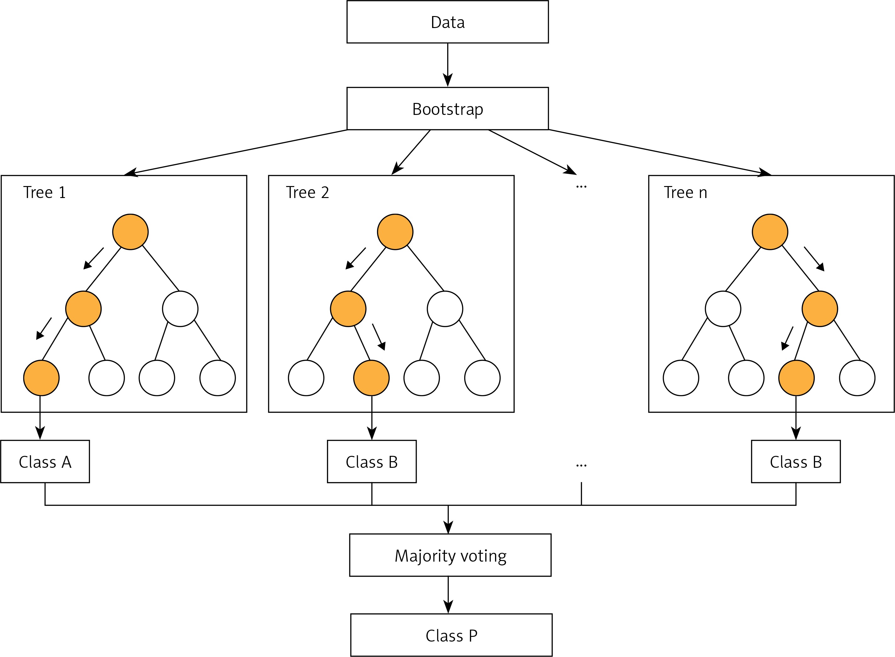
In fact, it is equivalent to sampling the samples and features (if the training data are regarded as a matrix, as is common in practice, then it is a process of sampling both rows and columns), so overfitting can be avoided.
OOB data weighted random forest (OOBWRF)
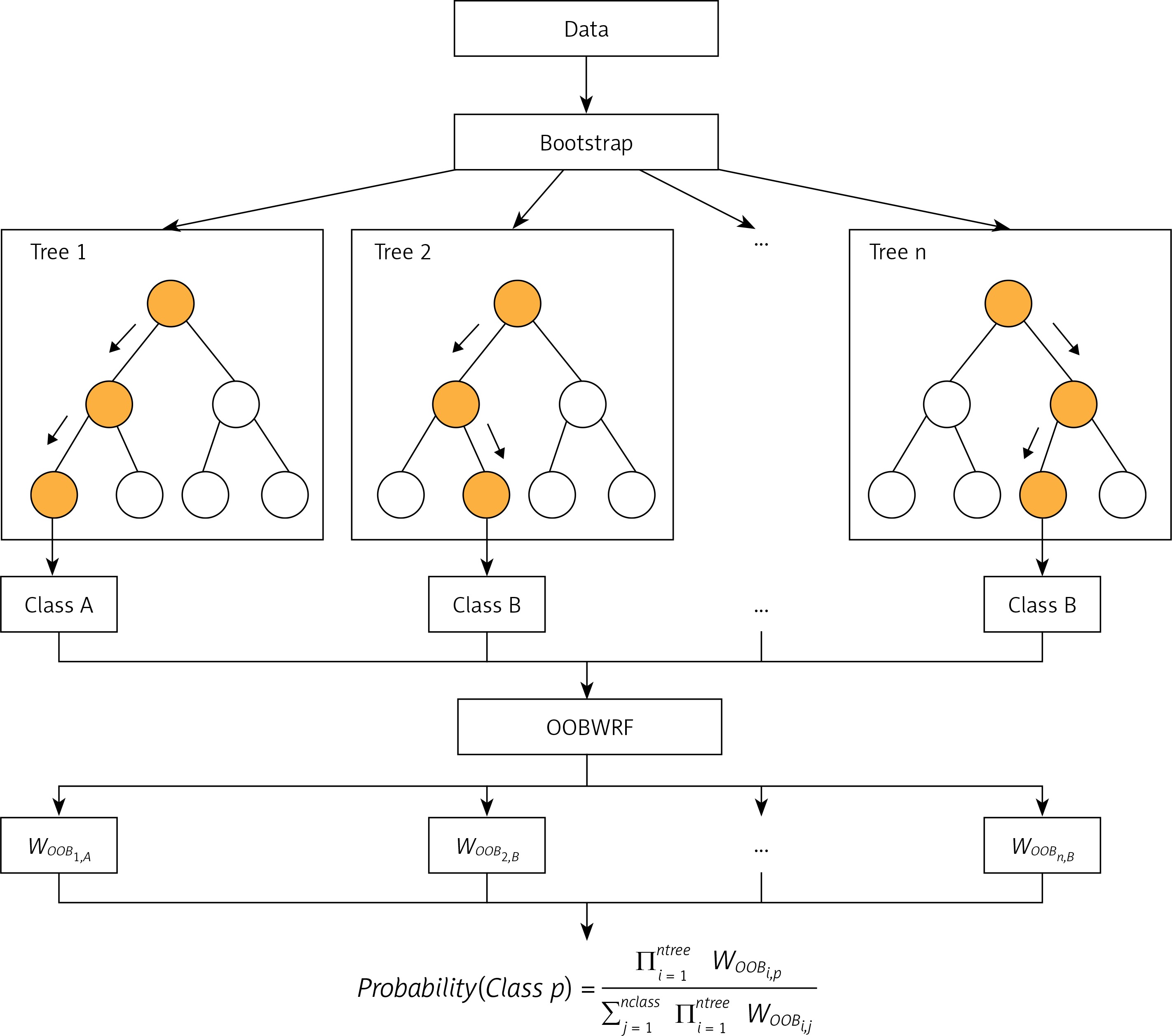
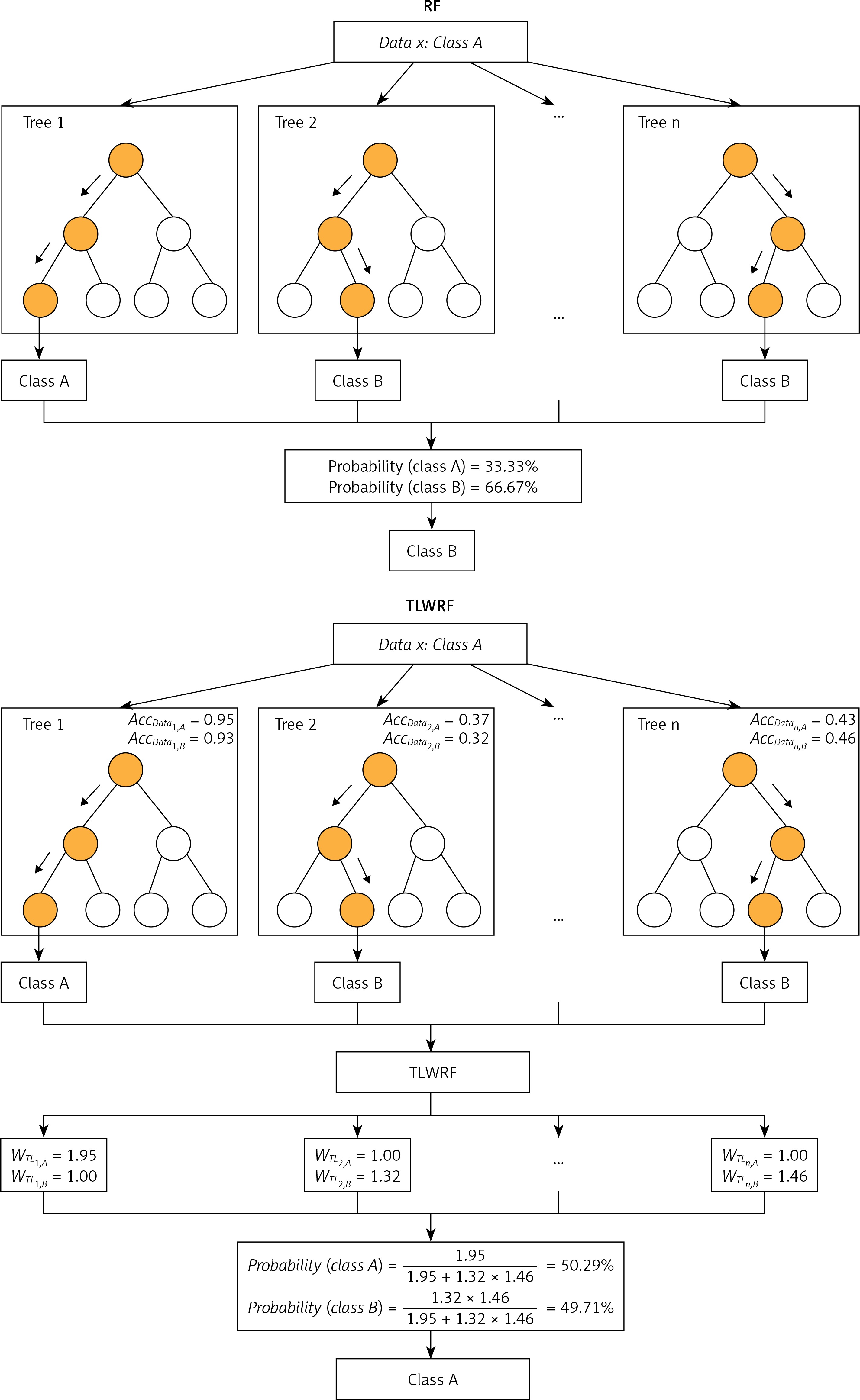
Using OOB data to evaluate DT in RF and using it as weighting is a universal strategy in RF weighting improvement. The principle is to improve the majority voting part of the RF model, instead of assigning the same weight to each tree as the original RF model. Because OOB data are not used in the process of fitting DT, it is feasible to use OOB data to evaluate the generalization performance of DT. We believe that it is reasonable to give a higher vote weight to DT with better generalization performance, so we weighted the majority voting process according to the accuracy tested by class using OOB data for each tree in the forest, and called this weighting method OOBWRF (Figure 2). The specific operation steps of using OOB data to weight and improve RF are in Equations 4, 5, 6, where AccOOBn,p represents the generalization performance of class p using OOB data to detect the nth tree, WOOBn,p represents the weight of class p of the nth tree, and predictionn represents the predicted result of the nth tree. The probability of predicting class p by the OOBWRF model is defined in Equation 6.
Tree-level weighted random forest (TLWRF)
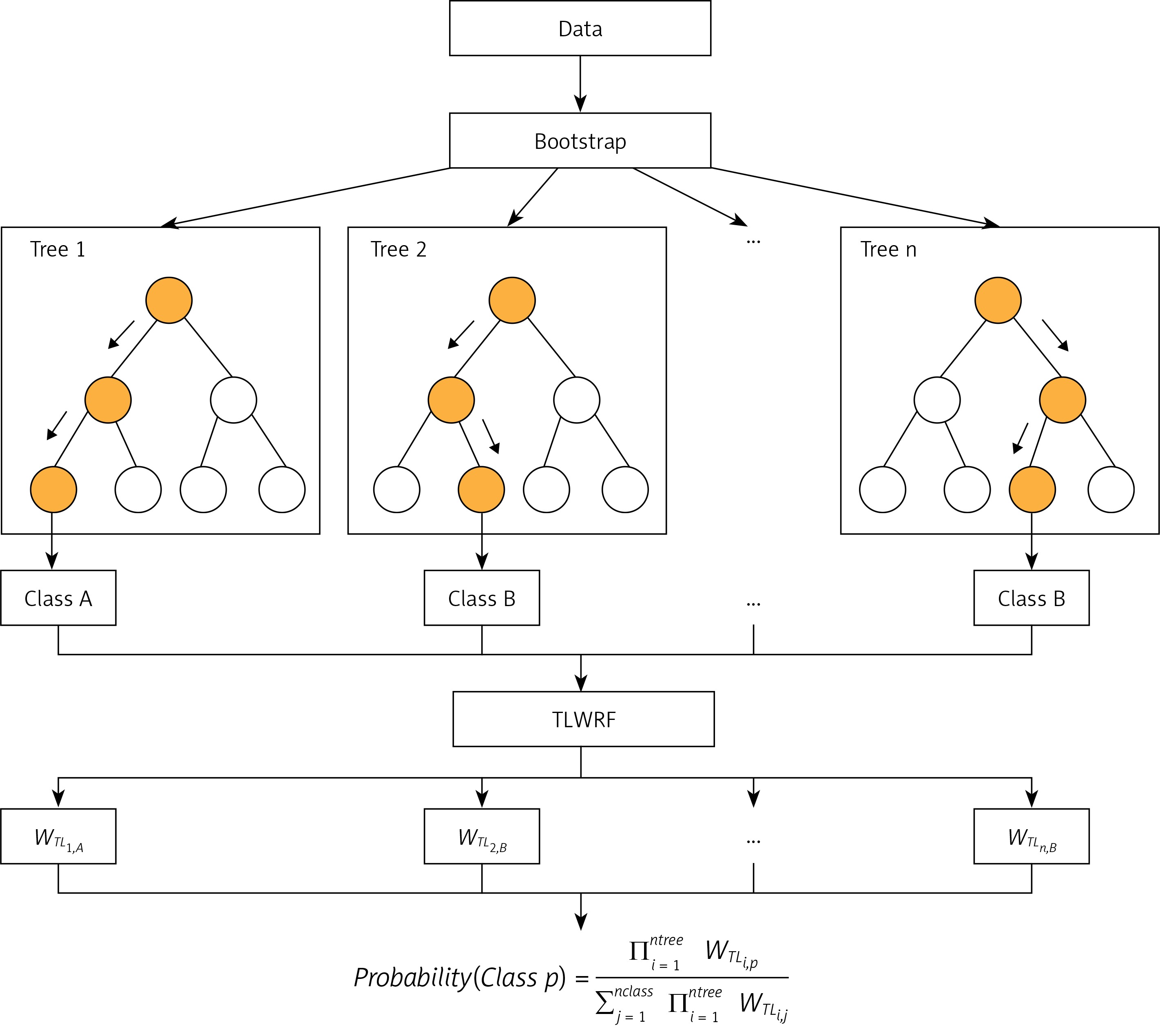
After rigorous experiments and analysis on the OOBWRF weighting method, we found that since the OOB data used to evaluate each tree are randomly generated through the bootstrap step in RF, the OOB data of each tree are different, so there are certain problems with the validity of the weights used for weighting, and the problem is found to be very serious through experimental results. In response to the above problems, based on the weighting framework of OOBWRF mentioned above, combined with the defects of using OOB data to weight, we propose TLWRF (Figure 3), which is defined in Equation 7, 8, 9. Replace the OOBn data used to evaluate each tree with the total training data Datan, and rename the p class weight of the new nth tree as WTLn,p in Equation 8.
Algorithm analysis
Although the above formula has clearly explained how the algorithm works and how to improve the original algorithm, a set of formulas do not intuitively let the reader understand how it works in a short period of time. So we use an example to describe how the model works ideally. We compare the original RF algorithm with our proposed TLWRF, this comparison is only to more intuitively show how TLWRF works, without any evaluation of the comparison results, and we only took out three trees in the forest for comparison. The comparison result is shown in Figure 4.
Results
Performance measures
A proper evaluation is crucial for models built with any statistical learning algorithm. In this experiment, we used accuracy and area under the receiver operating characteristic curve (AUC) as the performance evaluation methods of the model. Accuracy is the most basic performance evaluation index, but it is easily affected by the sample distribution, and it cannot well measure the performance of the model, so we introduced AUC as a supplement. We give the definition of accuracy in Equation 10. The receiver operating characteristic curve (ROC) is a curve drawn with different threshold points on the axes of TPR (true positive rate) and FPR (false positive rate). AUC is the area under the ROC curve. AUC is defined in Equation 11, where M and N are the number of positive and negative samples, while ranki indicates that the probability score of all samples are arranged from small to large, and the serial number of the i th sample.
In the process of testing multi-classified datasets, AUC will be averaged in two ways, micro and macro. In Experiment I, we give the AUC, based on these two averaging methods respectively, while in Experiment II, since both binary and multi-classified datasets are involved, we only list the AUC, under the macro averaging method in order to have a unified reference standard for the performance evaluation of the model.
Experiment I
In the treatment of cancer patients, it is extremely important to predict the survival status of patients according to their prognosis. Experienced doctors will evaluate the survival of patients based on their own experience through the medical index data of patients, but this is very difficult in countries and regions with an underdeveloped medical industry, so it is a very efficient means to realize the evaluation of patients through machine learning technology. We used TLWRF to fit the data of 110 697 cases of gastric cancer patients diagnosed from 1975 to 2016 obtained from the SEER database, so as to obtain a model that could predict the survival status of patients, and compared it with DT, RF and OOBWRF to verify that TLWRF played a role in improving the performance of the model in this experiment.
The cases evaluated in this analysis were extracted from the SEER-18 registry [26]; in order to achieve this, SEER*Stat software (Version 8.3.5) was used. The date of SEER data submission was November 2018. We introduced the Cox regression model to summarize the data in Equation 12, where β1, β2, …, βm is the partial regression coefficient of the independent variable; it is the parameter to be estimated from the sample data; h0(t) is the benchmark hazard rate of h(t, X) when the X vector is 0; it is the quantity to be estimated from the sample data. The Cox regression model is used to analyze the characteristics of patient data, and the details of the analysis results are shown in Table II. Through this table, the characteristics of the data can be understood objectively and directly. The coef attribute in Table II is β in the Cox regression model, and exp(coef) is commonly called the hazard ratio (HR). In cancer research, HR < 1 is called a good prognostic factor, while HR > 1 is called a bad prognostic factor. Considering the attributes in the table, especially the p-value and HR, we obtain the following conclusions about this data set, and this will provide an important reference for model evaluation after we use machine learning methods for modeling. All attributes except PRCDA 2016, sequence number, and total number of benign/borderline tumors for patient have a p-value of less than 0.005, which means that most attributes are expressed significantly. Among them, male patients have a 7% higher probability of death than female patients; total number of in situ/malignant tumors for the patient had a 12% negative impact on HR; stage group can reflect the patient’s survival status to the greatest extent compared to other attributes; patients with primary tumors have a 14% lower risk of death than patients with secondary tumors; marital status and histological grade both had a 6% impact on HR.
Table II
Details of the results of data characteristics analysis of gastric cancer patients based on Cox regression model (n = 110 697)
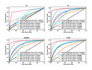
We carry out the preprocessing steps of vacant value processing, numerical replacement, one-hot encoding and so on. Considering the incomplete record of surviving patient data, only the data of deceased patients were used in the modeling process (n = 95648). Considering the imbalance of data target attribute distribution, we introduced the synthetic minority oversampling technique (SMOTE) algorithm for overfitting the data [27], and the data target attribute distribution after processing is the same (n = 328 988). According to the survival time of patients, the target classification attribute was calculated in terms of 3 years, 5 years, 10 years and over 10 years. Details of target attribute are shown in Table III, and this attribute is taken as the prediction target. The segmentation of the training set and the test set is such that 70% of the data is used for model training and 30% of the data is used for model validation. For all ensemble learning models, we conduct experiments on the base learner according to the number of 100. The experimental result data are shown in Table IV, and the details of the ROC curve of each model are shown in Figure 5.
Table III
Details of target attribute distribution
| Variable | 3 Years | 5 Years | 10 Years | >10 Years |
|---|---|---|---|---|
| Original n = 95 648 | 82247 (85.99%) | 4836 (5.06%) | 4754 (4.97%) | 3811 (3.98%) |
| Oversampled n = 328 988 | 82247 (25.00%) | 82247 (25.00%) | 82247 (25.00%) | 82247 (25.00%) |
Table IV
Experimental I results of OOBWRF and TLWRF compared to DT and original RF. The best-performing classifier for each evaluation index is highlighted
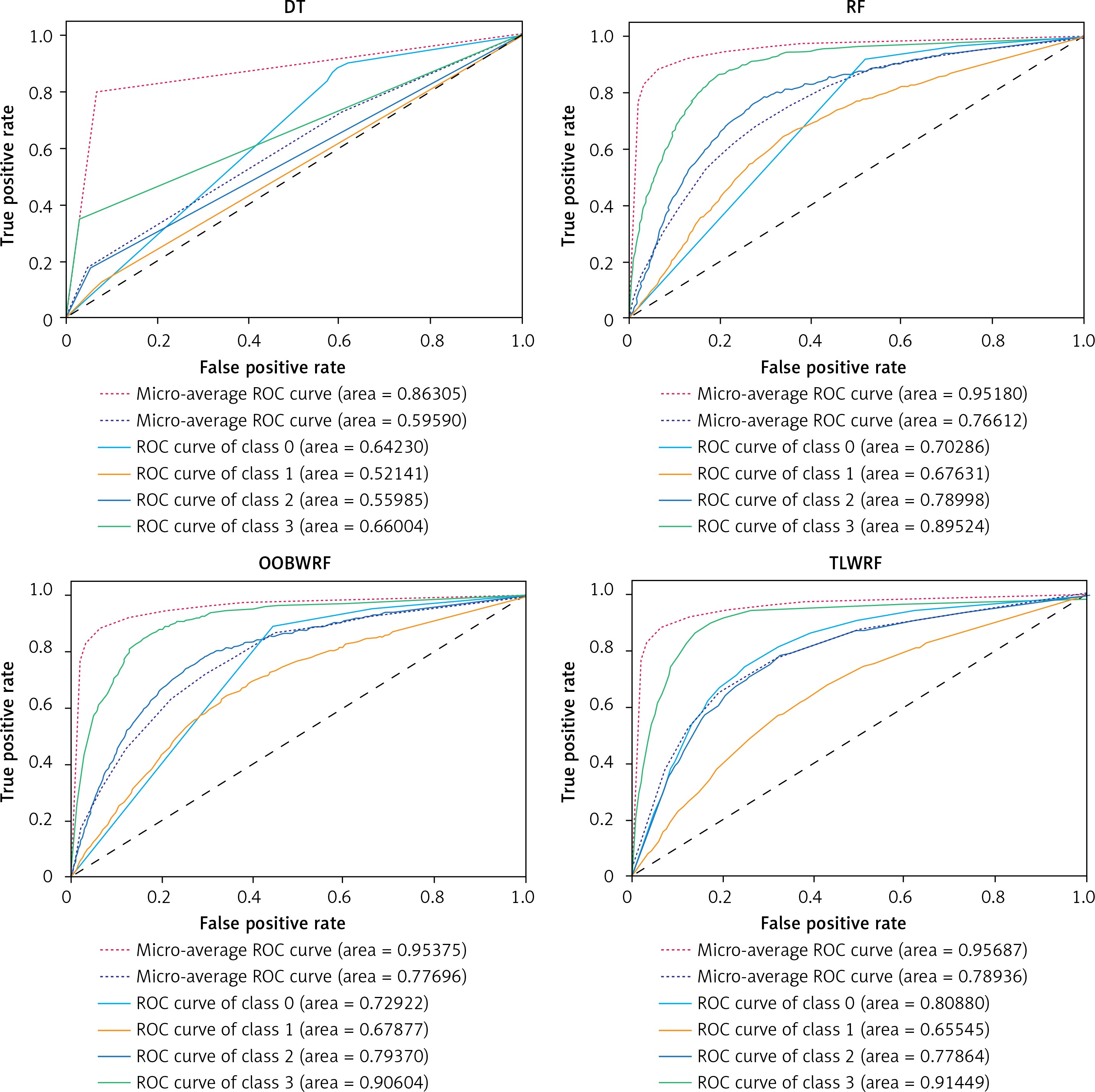
It can be learned from Table IV that compared with the original RF model, the two weighted models we proposed have been improved for all evaluation indexes. Among them, OOBWRF and TLWRF are 0.43% and 0.79% higher than RF in accuracy, respectively. In the AUC index, it is increased by 2.63% and 10.59% in Class 0, 0.25% and –2.09% in Class 1, 0.37% and –1.13% in Class 2, and 1.08% and 1.93% in Class 3, respectively. On the two average AUCs, macro increases by 1.08% and 2.32%, respectively, and micro increases by 0.2% and 0.51%, respectively.
Overall, the TLWRF we proposed is the best performing model compared to the other three listed models. We believe that through our experiment, doctors and patients will have a clearer understanding of the condition of gastric cancer from the perspective of machine learning. Only relevant indicators of the patient’s condition can be used to make use of this more accurate model. So we think this experiment is meaningful, especially for those areas with an underdeveloped medical level and inexperienced doctors.
Experiment II
In order to verify that the performance of TLWRF has been improved based on the original model, we obtained 10 public medical datasets from the UCI machine learning repository [28] to verify the performance of the model, including 7 binary datasets and 3 multi-classification datasets. The details of the datasets used are given in Table V.
Table V
Details of the test datasets downloaded from the UCI machine learning repository
The datasets used all go through data preprocessing steps such as numerical replacement and missing value processing. 70% of the data set is used for model training and 30% for model verification. The tool used for the simulation experiment is sklearn (version 0.23.1), using train_test_split to divide the data into a training set and test set. The base learners used are 100 decision trees. The oob_score parameter is set to true, and the rest of the parameters are RandomForestClassifier’s default parameters. In the course of the experiment, all the parameters that need to be used for random control, such as random_state, are set to 0 to ensure that the experimental results can be reproduced.
Accuracy and AUC mentioned in the Performance Measures section are used as evaluation indexes for the experiment. The two indexes will be listed respectively and the model with the highest score will be highlighted in Table VI.
Table VI
Experimental II results of OOBWRF and TLWRF compared to DT and original RF. The best-performing classifier for each dataset is highlighted according to accuracy and AUC. The last row shows the average accuracy of all models considering all datasets
The performance of the four models on 10 public datasets can be seen from Table VI. In the accuracy index, the number of DT with the highest score was 0/10, with an average score of 74.93%; the number of RF with the highest score was 1/10, with an average score of 79.98%; the number of OOBWRF with the highest score was 3/10, with an average score of 77.83%; the number of TLWRF with the highest score was 9/10, with an average score of 81.42%. Compared with RF, the average accuracy OOBWRF decreased by 2.15%, and average accuracy TLWRF increased by 1.44%. In the AUC index, the number of DT with the highest score was 0/10, with an average score of 72.94%; the number of RF with the highest score was 4/10, with an average score of 85.78%; the number of OOBWRF with the highest score was 1/10, with an average score of 84.27%; the number of TLWRF with the highest score was 6/10, with an average score of 86.98%. Compared with RF, the average AUC OOBWRF decreased by 1.51%, and average AUC TLWRF increased by 1.2%.
Discussion
In view of the defect that the random forest model assigns the same weight to all base learners, we proposed a weighting strategy for base learners, and used this strategy to propose two improved models, TLWRF and OOBWRF. From the numerical results, two weighted models, OOBWRF and TLWRF, are both of practical significance. The performance of TLWRF in Experiment I and Experiment II is the best among the four models listed.
In Experiment I, we used the TLWRF proposed in this paper to model the data of 110 697 patients with gastric cancer obtained from the SEER database, and got a better modeling method than the original random forest algorithm. It is meaningful for the integration of medicine and machine learning. A more accurate model will be obtained by using our improved algorithm, so as to improve the accuracy and efficiency of diagnosis. Through some medical indicators of patients, the prognosis of patients can be predicted and analyzed quickly. Meanwhile, we obtained 10 public medical datasets from the UCI machine learning repository to test and compare the generalization performance of each model in Experiment II. The results show that our proposed model can not only improve the data modeling of gastric cancer patients, but also improve the performance in other medical classification tasks. And through these two experiments, we also reach the following two conclusions:
Weighting the base learners of random forest according to their performance is an effective method to improve the defects of random forest;
From the experimental results, unlike the customary use of OOB data test results as a weighted basis, we tend to use the test results of all training data as a weighted basis, because models that use this basis generally produce better performance.
Admittedly, because the machine is not affected by individual subjective factors, doctors with high level medical training will introduce advanced artificial intelligence or machine learning methods into daily diagnosis and treatment as one of the reference indicators. This is particularly important under the influence of COVID-19 virus all over the world. Artificial intelligence and machine learning technology will be more and more irreplaceable in the development of medicine in the future. Nevertheless, in the field of medicine, artificial intelligence and machine learning are not so reliable today, although it is believed that this situation will be improved in the future.
According to this research, we believe that more studies that may be carried out in the future include:
A user-friendly medical auxiliary decision platform that can be practically used is built using the achievement of this research.
Exploring the influence of the parameters in the random forest model on the weighted random forest model;
Combining other machine learning models to integrate the random forest weighting method;
Combine pruning and weighting to better improve the performance of random forest;
More weighting methods, etc.