Introduction
Diabetes is a chronic metabolic disorder characterized by abnormal blood sugar levels, caused by improper use of insulin or insufficient insulin secretion, leading to severe long-term damage to multiple organs and body systems (including kidneys, heart, nerves, blood vessels, and eyes) [1], ultimately becoming a major contributor to mortality [2]. On a global scale, diabetes has become a daunting public health challenge, with its prevalence continuing to rise [3]. From 2021 to 2050, the global burden of diabetes will rise from 529 million to 1.31 billion people [4]. Despite the projected dramatic increase in the future diabetic population, high-risk individuals often underestimate their own risk of developing the disease [5, 6]. Once high-risk individuals progress to confirmed cases, although there are treatment methods available to slow down the progression of the disease, there is still a lack of curative treatment options [7]. Considering the high prevalence of diabetes and the relatively large size of the high-risk population [8], it is crucial at a population level to further identify risk factors and take preventive measures before high-risk individuals develop the disease state [9].
In recent years, the application of machine learning techniques in the medical field has become increasingly widespread, especially in the prediction of disease risks and diagnosis, exhibiting potential value [10–12]. Utilizing rich clinical data and advanced algorithms, machine learning studies based on large-scale databases have become a hot topic in diabetes research, aiding in identifying individuals at risk of diabetes and providing personalized prevention and management strategies [13, 14]. For example, a project used five machine learning models – Logistic Regression, Support Vector Machine, Random Forest (RF), Extreme Gradient Boosted Tree, and Weighted Voting Classifier – to predict diabetes in adolescents and identify factors leading to diabetes in adolescents, such as waist circumference, gender, BMI, and leg length [15]. However, research on the risk assessment of diabetes in high-risk populations has not been fully developed yet.
Therefore, this project utilized the National Health and Nutrition Examination Survey (NHANES) database with a large sample size to develop a machine learning-based diabetes risk prediction model for high-risk populations. The model was designed to enable early identification of individuals at high risk of diabetes within high-risk populations, facilitating timely preventive and therapeutic interventions. This research is of great significance for reducing the incidence of diabetes and related complications.
Material and methods
Data source and study population
This investigation conducted data analysis using the NHANES public database, which was established and continuously updated and improved by the Centers for Disease Control and Prevention (CDC) in the United States. The NHANES employs a layered, multi-stage probability sampling method to select a nationally representative sample of the population, and collects data through direct physical examinations, clinical and laboratory tests, personal interviews, and relevant measurement procedures. Relevant questionnaires and study protocols can be obtained from the NHANES official webpage on the CDC website [16]. The NHANES has obtained ethical approval from the National Health Statistics Research Ethics Review Committee in the United States, and all participants have signed informed consent forms to ensure that they understand and agree to participate in the survey.
Participants
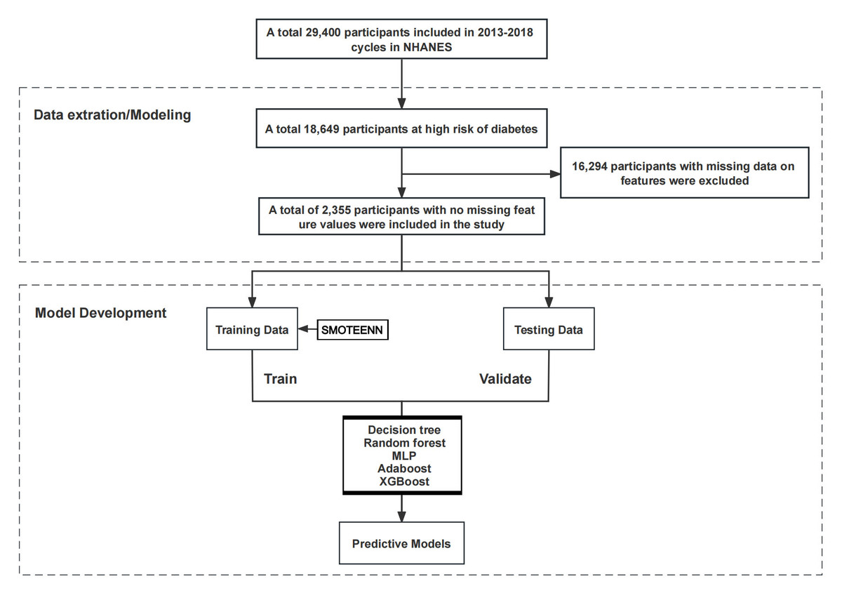
In this project, we selected a sample of individuals at high risk of diabetes from 29,400 participants in the NHANES from 2013 to 2018. The definition criteria for high-risk groups of diabetic patients were those who meet any of the following conditions: (1) age ≥ 40 years old; (2) impaired glucose tolerance (fasting glucose < 126 mg/dl and 140 mg/dl ≤ OGTT (oral glucose tolerance test) < 200 mg/dl) [17] or abnormal fasting glucose (100 mg/dl ≤ fasting glucose < 126 mg/dl) [18]; (3) overweight (BMI ≥ 25 kg/m2); (4) lack of physical activity (moderate or equivalent intensity activity time < 150 min per week); (5) family history of diabetes; (6) a history of gestational diabetes; (7) high blood pressure or taking antihypertensive drugs; (8) a history of coronary heart disease; (9) patients with polycystic ovarian cancer syndrome; (10) taking antidepressants for more than 3 months and depression diagnosed by ICD-10 coding (F32.9 and F33.9). By applying the above screening criteria, 18,649 individuals at high risk of diabetes were identified. Subsequently, 16,294 samples with missing feature data were excluded, resulting in 2,355 eligible samples that met the criteria. These samples were divided into training and testing sets in a 7 : 3 ratio for the construction and evaluation of machine learning prediction models. The specific inclusion process is shown in Figure 1.
Outcome variables
Diabetes as the outcome variable was defined as meeting one of the following criteria: (a) diagnosed with diabetes by a doctor; (b) taking antidiabetic medication; (c) glycosylated hemoglobin HbA1c > 6.5%; (d) fasting blood glucose > 126 mg/dl [19, 20]. In this project, the outcome variable was defined as a categorical variable, encoded in numerical form for binary classification of high-risk individuals: 0 indicating non-diabetes and 1 indicating diabetes. Categorical features were encoded with numerical values for analysis.
Feature variables
The feature variables in this project included demographic baseline data, measurement data, medical history, and the Patient Health Questionnaire (PHQ)-9. Demographic baseline data included gender, age, race, education level [21], poverty-income ratio (PIR), and family history of diabetes. Measurement data included waist circumference, BMI, diastolic blood pressure (DBP), and systolic blood pressure (SBP). History of disease included heart disease, hypertension, arthritis, cancer, stroke, hearing impairment, vision impairment, asthma, and kidney failure [22, 23]. Kidney failure was defined as eGFR ≤ 60 ml/min/1.73 m2 or albumin to creatinine ratio ≥ 30 mg/g [24]. Depression was assessed using the PHQ-9, which includes 9 items rated on a 0–3 scale (0 = “not at all”, 1 = “a few days”, 2 = “more than half the days”, and 3 = “almost every day”), yielding a total score of 0–27 points [25, 26].
Machine learning
We applied five machine learning algorithms to train the classification model. The first one was the decision tree, a classification model based on a tree-like structure, which was used to make decisions by progressively splitting the data into multiple nodes. The decision tree model is easy to understand and interpret, and suitable for handling non-linear relationships and complex rules in data [27]. Random forest (RF) is an ensemble learning model that reduces errors and improves prediction reliability by constructing multiple independent decision trees (similar to a flowchart judgment model) and then synthesizing the results of all trees [28]. Multilayer perceptron (MLP) is a network model that simulates the connections of human brain neurons. By continuously adjusting the connection strength of each neuron in the network (i.e. a backpropagation algorithm), it reduces prediction errors and improves the ability to judge disease risk [29]. Adaboost, an ensemble learning method, can first train a simple model (weak classifier), then adjust weights based on its incorrectly predicted samples (making hard-to-predict samples more noticeable), and then train the next model, ultimately integrating the results of all models to improve prediction accuracy [30]. XGBoost, an efficient gradient boosting algorithm that continuously builds new decision trees to correct errors in previous models, can gradually improve predictive performance. It is suitable for processing complex data and is widely used in classification and regression tasks, with great performance on large-scale datasets [31].
Statistical analysis
Continuous variables were presented in the form of mean and standard deviation, while categorical variables were presented as percentages. We used the t-test for inter-group comparison of continuous variables and a χ2 test for inter-group comparison of categorical variables. The data were split into a 7 : 3 ratio for training and testing sets. Machine learning models were developed using Python 3.9.7 and the sklearn package [32], and the receiver operating characteristic (ROC) curves were plotted using the matplotlib package [33]. Five machine learning algorithms – Decision Tree, RF, MLP, Adaboost, and XGBoost – were applied to train the prediction model. The grid search method was employed to generate the optimal model parameters by adjusting the model parameters for different models and evaluating their performance. The trained models were evaluated on a test set using 10-fold cross-validation to determine the stability of the model. The following indices were used in evaluation: accuracy (the proportion of correct overall model predictions), sensitivity (the ability to correctly identify actual patients, that is, the proportion of “no missed diagnosis”), specificity (the ability to correctly identify actual unaffected individuals, that is, the proportion of “no misdiagnosis”), the area under the curve (AUC) of the ROC curves (the comprehensive ability of the model to distinguish between diseased and non-diseased individuals, with a value closer to 1 indicating greater ability to distinguish patients), and the Matthews correlation coefficient (MCC), the accuracy of model classification, ranging from –1 to 1, with the value closer to 1 indicating the more reliable ability of classification). Based on the best-performing machine learning model, the SHAP (SHapley Additive exPlanations) model, a tool grounded in mathematical theory, was used to analyze the impact of each factor on the model’s prediction results, identifying more important factors for diabetes risk prediction. The partial SHAP values were plotted as a summary plot, which included the relative ranking of features and the relationship between each feature and the outcome. The SHAP values for each feature were calculated for each sample to reflect the impact of the feature on the prediction result. Next, we aggregated the average absolute SHAP values and summarized the global contribution of each feature in a bar chart form [34]. To address the issue of data imbalance in the study, the combination technique of SMOTEENN from the imblearn package was applied to handle imbalanced data. First, we oversampled SMOTE, then cleaned the samples with the edited nearest neighbors (ENN) method to reduce noisy samples and refine model generalization performance [35] (p < 0.05: statistically significant).
Results
Baseline characteristics
The baseline characteristics included in this project are presented in Table I. With 260 diabetic patients and 2,095 non-diabetic patients in high-risk groups, the results indicated that the average age of those with diabetes was higher (46.37 vs. 39.15, p < 0.001), and the proportion of people with a high school education level or equivalent was lower compared with the non-diabetic group (46.9% vs. 48.4%, p = 0.020). Waist circumference (113.35 vs. 99.32, p < 0.001) and SBP (126.22 vs. 121.06, p < 0.001) in diabetic patients were significantly higher than those in the unaffected group. Heart disease (9.6% vs. 4.2%), hypertension (68.5% vs. 46.0%, p < 0.001), arthritis (35.4% vs. 20.9%, p < 0.001), stroke (35.4% vs. 20.9%, p < 0.001), asthma (25.0% vs. 18.5%, p = 0.016), chronic kidney disease (23.5% vs. 9.3%, p < 0.001), hearing loss (11.5% vs. 9.3%, p < 0.001). 5.5%, p < 0.001), and visual loss (12.7% vs. 5.6%, p < 0.001) were more likely to occur in diabetic patients than in unaffected people. In addition, patients with diabetes also showed elevated scores of PHQ-9 (5.50 vs. 5.06, p = 0.01).
Table I
Characteristics of NHANES participants
Model performance comparison
Table II shows the performance of five models on the test set. The decision tree model had an accuracy of 0.744, sensitivity of 0.714, specificity of 0.789, and AUC of 0.751. In contrast, the RF model had an accuracy of 0.784, sensitivity of 0.739, specificity of 0.849, and AUC of 0.896, exhibiting better performance in all aspects. The MLP model had an AUC of 0.900 on the test set, with high accuracy (0.822) and sensitivity (0.905), but slightly lower specificity (0.704). The AUC of the AdaBoost model on the test set was 0.895, with a specificity of 0.805 and good accuracy (0.837) and sensitivity (0.859). The XGBoost model had an accuracy of 0.815, sensitivity of 0.962, specificity of 0.602, and AUC of 0.903 on the test set. Compared to MLP and AdaBoost, the XGBoost model had lower specificity but possessed the best sensitivity and classification ability.
Table II
Results from 10-fold cross-validation for diabetes classification
Additionally, we calculated the MCC for each model to provide a more comprehensive evaluation of model performance. As shown in Table II, the MCC for the decision tree model was 0.361, for the RF model was 0.418, for the MLP model was 0.447, for the Adaboost model was 0.463, and for the XGBoost model was 0.443. The results indicated that the Adaboost and MLP models performed well in balancing sensitivity and specificity. However, the MCC results further supported the conclusion that the RF and XGBoost models excelled in classification accuracy and recognition capability, respectively. The MCC values of these two models still demonstrated their good classification capabilities. Therefore, from an overall assessment of model performance, RF and XGBoost were the top-performing models.
Feature importance
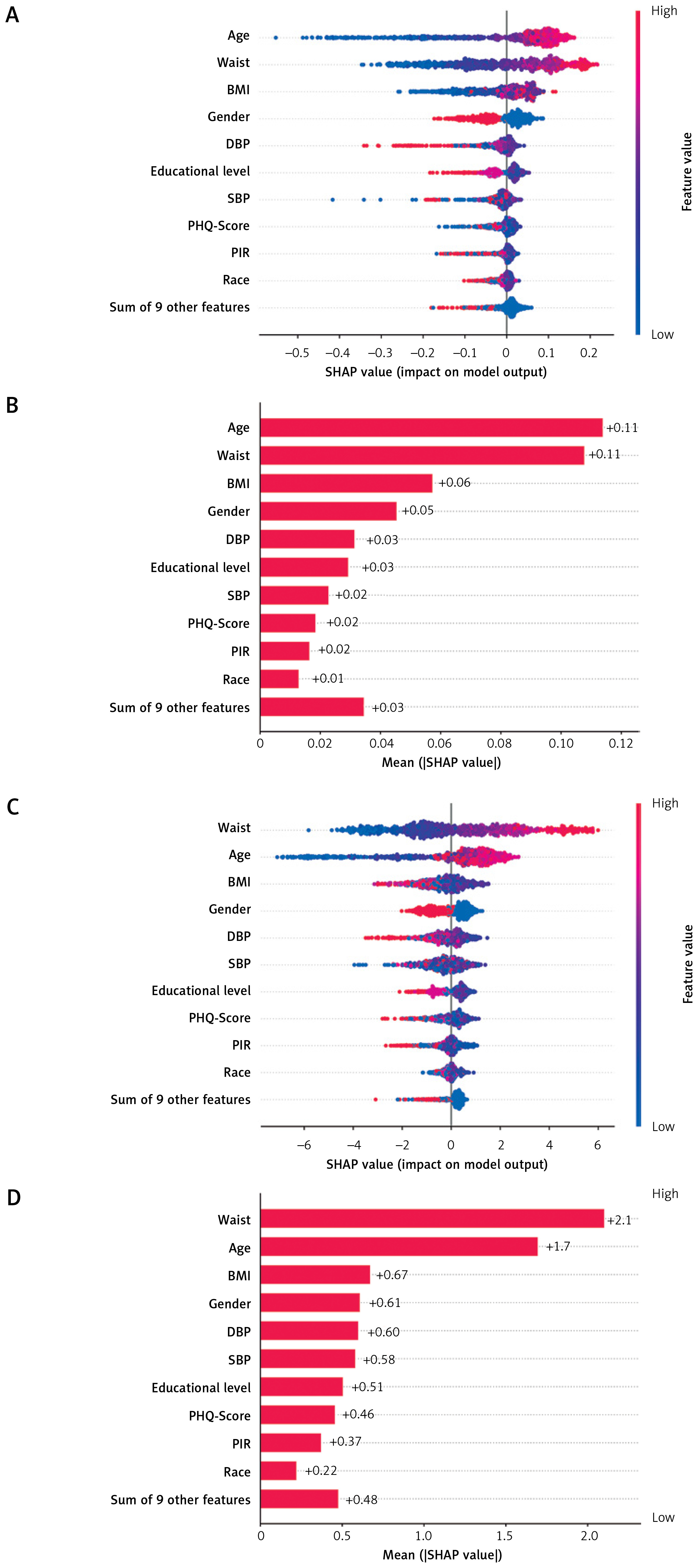
Based on the comparison of model performance above, we employed RF and XGBoost to calculate the importance of each feature. Figure 2 shows the impact of the baseline values of the top 10 features on the model output, i.e., the development of relative risk for diabetes. Combining the SHAP summary plot (Figure 2 A) with the bar plot (Figure 2 B), the top three features in the RF model were age (SHAP = 0.11), waist circumference (SHAP = 0.11), and BMI (SHAP = 0.06), while sex, DBP, education level, SBP, PHQ-9 score, PIR, and race were the next most important features. Similarly, in the XGBoost model, the top three features were waist circumference (SHAP = 2.1), age (SHAP = 1.7), and BMI (SHAP = 0.67), while sex, DBP, SBP, education level, PHQ score, PIR, and race were the next most important features (Figures 2 C, D). In the RF and XGBoost models, waist circumference, age, BMI, and PHQ-9 score were positively correlated with diabetes risk, while education level and PIR were negatively correlated with diabetes risk, and women had a higher diabetes risk relative to men.
Figure 2
Summary plot and feature importance for SHAP values in the testing set. Summary SHAP plots (A) and bar plots (B) of the global SHAP values of the RF model. Summary SHAP plots (C) and bar plots (D) of the global SHAP values of the XGBoost model. SHAP summary plot provides three aspects of information: (1) ranking indicates the relative importance of features; (2) Color gradients indicate the relative size of each feature, with red indicating high values of the feature (e.g., older age) and blue indicating the opposite (e.g., younger age), where females are shown in blue and males in red. A negative SHAP value indicates a decreased relative risk, whereas a negative SHAP value indicates an increased relative risk. (3) The discretization of points indicates whether the relationship between each feature and the outcome is linear. The bars show the global SHAP values
PIR – poverty income ratio, DBP – diastolic blood pressure, SBP – systolic blood pressure, PHQ – Patient Health Questionnaire.
Discussion
In this project, 2,355 individuals at high risk of diabetes from the NHANES dataset in the years 2013–2018 were included to develop the risk model. We applied five machine learning methods (decision tree, RF, MLP, Adaboost, and XGBoost) and evaluated their performance, finding that the AUC values of the RF and XGBoost models in the test set were 0.896 and 0.903, respectively. The accuracy of the RF model on the test set was 0.784, with sensitivity of 0.739 and specificity of 0.849, while the XGBoost model had an accuracy of 0.815, with sensitivity of 0.962, indicating that these two machine learning algorithms possessed high predictive ability in diabetes risk assessment. Moreover, the MCC values of the RF and XGBoost models were 0.418 and 0.443, respectively, further validating their robust classification performance when handling imbalanced datasets. This also reinforces the suitability of RF and XGBoost for developing personalized diabetes risk assessment tools. Furthermore, we also conducted feature importance analysis on these two models and found that waist circumference, age, and BMI were closely linked to the development of diabetes, while gender, SBP, DBP, education level, PIR, PHQ score, and race were identified as important predictive factors. The present work provided important insights for innovating personalized disease risk assessment tools in the future, with great potential to refine the early prevention and management of diabetes.
In this study, XGBoost performed the best in overall performance with its gradient boosting architecture, which is consistent with the conclusions of multiple studies. For example, XGBoost achieved an AUROC of 0.92 in health literacy prediction and nutrition score modeling, outperforming RF (0.90) and logistic regression (0.88), and leading in sensitivity (91%), specificity (84%), and other indicators [36]. Another NHANES study showed that the AUC of XGBoost (0.8168) was significantly higher than that of RF and logistic regression (about 0.79), and the three were similar in accuracy (about 85%) [37]. In addition, in the Patient Generated Subject Global Assessment (PG-SGA) score prediction, the AUC values of XGBoost and RF were 0.75 and 0.77, respectively, showing the best performance [38]. The high sensitivity of XGBoost (> 96% in this study) makes it an ideal tool for preliminary screening of large-scale populations, minimizing missed diagnosis rates to the greatest extent possible. In contrast, although RF has slightly lower AUC (0.896) and sensitivity (0.739) than XGBoost, its specificity (0.849) is significantly higher. This “low false positive” advantage stems from its ability to capture non-linear relationships and feature interactions [39]. Therefore, the RF model is more suitable for clinical diagnosis, such as conducting secondary validation on individuals with XGBoost initial positive screening to reduce misdiagnosis rates and avoid wasting limited medical resources on false-positive individuals. This two-stage strategy (XGBoost preliminary screening + RF verification) can be effectively integrated into the existing management process of high-risk groups of diabetes. More specifically, the XGBoost model is used to quickly identify a large number of potential high-risk individuals in community physical examination, health file system organization, or outpatient preliminary screening. Subsequently, for those who tested positive in the initial screening, the RF model was applied in the clinical environment for more accurate review and risk assessment, and intervention priorities were determined based on the doctor’s judgment. It is worth noting that traditional models still have value in specific scenarios. Logistic regression often performs robustly in external validation sets. In comparisons of models such as Bayes logistic regression and decision trees, logistic regression repeatedly ranks among the top three [40], but its performance may be limited when dealing with nonlinear relationships [41]. Meanwhile, support vector machines (SVM) are comparable to the optimal model in certain tasks (such as AUROC 0.83) [42], but most studies show that their performance is slightly inferior to RF or XGBoost [43, 44].
This study found that BMI, age, waist circumference, and depression were positively correlated with diabetes in high-risk groups, and these key predictors were highly consistent with the existing literature on diabetes risk. Firstly, waist circumference, as a core index to measure abdominal obesity, was identified as the most important predictor (the highest SHAP value) in the RF and XGBoost models of this study, which is consistent with a large body of evidence that abdominal visceral fat is the core pathophysiological mechanism of diabetes [45]. The visceral adipose tissue has strong metabolic activity and secretes a large amount of pro-inflammatory factors and free fatty acids, directly leading to insulin resistance and β-cell dysfunction [45, 46]. Secondly, age, as a non-modifiable risk factor, has been consistently associated with the development of disease [47, 48]. This study again supported the key role of β-cell function decline and insulin sensitivity decline in the development of diabetes during aging [49, 50]. Thirdly, as an indicator of overall obesity, BMI has a strong association with diabetes [51–53]. This study confirmed that BMI is still an important risk marker in high-risk groups. Obesity (whether overall or abdominal) promotes the development of diabetes by increasing pancreatic fat deposition, increasing the burden of β cells, and systemic insulin resistance [54, 55]. Finally, this study found that depression is an important psychosocial risk factor, which is consistent with previous research [56, 57]. It is worth noting that this study not only confirmed the risk of depression, but also included the screening criterion of “continuous use of antidepressant drugs for more than 3 months.” The results also suggest that this population has a higher risk, which is consistent with the literature exploring the possible impact of antidepressant drug use on blood glucose control [58].
The positive correlation of BMI, age, waist circumference, and depression with the risk of diabetes in high-risk groups not only provides strong support for the study of diabetes risk mechanisms but also has a clear application value in clinical practice and public health. From the perspective of clinical practice, these key predictors can directly guide the hierarchical management and precise intervention of high-risk groups. First, waist circumference can be included in the core indicators of routine screening of high-risk groups of diabetes in clinical practice, and individuals with markedly high waist circumference should be prioritized for in-depth tests such as fasting blood glucose and glycosylated hemoglobin. At the same time, targeted abdominal fat reduction programs should be developed, such as combining diet control and core muscle group training, to reduce the risk of insulin resistance caused by visceral fat deposition [59]. Secondly, in response to the non-modifiable risk factor of aging, in clinical practice, it is necessary to strengthen regular follow-up for high-risk populations over 40 years old, especially focusing on their blood glucose fluctuations and changes in β-cell function. Early initiation of lifestyle interventions can delay the decline of β-cell function. Thirdly, for individuals with high BMI, weight management should be the core intervention goal, achieved through personalized nutrition guidance and exercise prescriptions to reduce pancreatic fat burden and improve insulin sensitivity [60]. Fourthly, for high-risk populations with depression and long-term use of antidepressants, psychiatric and endocrinology departments should collaborate to evaluate and prioritize the selection of antidepressants with a minimal impact on blood sugar. At the same time, regular monitoring of glycated hemoglobin and fasting blood sugar should be conducted to avoid adverse effects of medication on blood sugar control. In addition, from the perspective of public health applications, a simple risk scoring tool can be developed based on waist circumference, age, BMI, and depression status to enable primary healthcare institutions to quickly identify high-risk individuals. For high-risk subgroups such as the elderly who are easily overlooked, theme health education should be implemented by combining community resources to lower intervention thresholds. For the population using long-term antidepressant therapy, medical institutions should establish a linkage mechanism between medication and blood glucose monitoring, and blood glucose indicators should be incorporated into the routine evaluation system for depression treatment [61]. Through a combination of clinical practice and public health measures, risk prediction can be transformed into active prevention to ultimately reduce the incidence rate of diabetes and the burden of related complications.
In this study, SBP and DBP were also found to be associated with the risk of diabetes. Multiple population studies have confirmed the universality of this association. Among African Americans and Caucasians aged 35–54, higher blood pressure is associated with a higher risk of diabetes compared with normal blood pressure [62]. The Korean adult cohort study showed that even for people in prehypertension (120–139/80–89 mm Hg), their risk of diabetes was significantly higher than that of normotension [63]. These studies indicate that blood pressure management should not be limited to patients with diagnosed hypertension. Blood pressure monitoring of high-risk groups (including early status) should be the core component of diabetes prevention strategies. In addition, race has been identified as a key sociobiological predictor. American data show that the prevalence of diabetes among non-Hispanic blacks, Asians, and Hispanics (12–14%) is significantly higher than that of other ethnic groups [64], and this difference persists among high-risk elderly people [65]. It suggests that when developing public health interventions, it is important to focus on high-risk racial/ethnic groups and integrate culturally sensitive support programs in community screening and health management.
In our study, women in high-risk groups showed a higher risk of developing diabetes compared to men. This is closely related to the physiological changes unique to women, especially the lack of estrogen during menopause. Premature menopause (< 40 years old) or surgical menopause significantly increases the risk of type 2 diabetes [66, 67]. Estrogen deficiency affects the development of diabetes through multiple mechanisms, including changes in insulin secretion of pancreatic β cells, decreased sensitivity of targeted organs and tissues to insulin, and increased sensitivity of major organs of diabetes-related pathology to glucose [67]. In addition, in an epidemiological study, the risk of insomnia in women of all ages was found to be generally 40% higher than that in men, and there is a close relationship between insomnia and diabetes [68]. Sleep disorders are closely related to obesity and insulin resistance [69]. Lack of sleep can disrupt key hormones that regulate appetite and energy balance (such as leptin, ghrelin, and adiponectin), increase intake of high-calorie foods, and worsen blood sugar control [70–72]. This suggests that diabetes risk screening should routinely include women’s reproductive history (such as menopausal age, surgical menopause history) and sleep quality evaluation. At the same time, for perimenopausal and postmenopausal women, weight management and education and support for lifestyle intervention (healthy diet, regular exercise) should be strengthened.
Education level and income are equally crucial social determinants. High levels of education typically promote healthier lifestyles, reduce shift work (lowering stress and obesity risk), and enhance health awareness and proactive prevention behaviors [73–76]. Conversely, low income and poverty significantly increased the risk of diabetes (the probability increased 2–3 times) [77]. Improving the socio-economic environment (such as moving out of high poverty areas) can reduce the prevalence of diabetes [78]. Poverty is often accompanied by resource limitations such as malnutrition and lack of safe exercise space, exacerbating risk factors such as obesity [79]. Therefore, for interventions in groups at high risk of diabetes, we must pay attention to improving the health literacy of low-education/low-income groups, and provide culturally appropriate and easy-to-understand educational materials and support services. At the same time, a sound social security system should be established to ensure their access to nutrition and basic medical services, and create a supportive environment to encourage physical exercise [80].
This study showed that the RF and XGBoost models had the best risk prediction performance among groups with high-risk diabetes, effectively identifying key risk factors such as waist circumference, age, BMI, depression, SBP, and DBP, as well as socioeconomic factors such as gender, education level, and income. These findings support the development of RF and XGBoost models as personalized risk assessment tools that can be embedded in electronic health records systems or mobile health applications to assist clinicians in achieving risk stratification management, improving the efficiency of early screening and intervention for diabetes, and ultimately reducing the incidence rate and burden of complications.
However, this study also has some limitations. Firstly, the study adopted a cross-sectional design and cannot directly infer causal relationships. Compared to longitudinal studies that can reveal the temporal correlation of disease occurrence through long-term follow-up data (such as tracking changes in blood glucose and dynamic evolution of risk factors), this study failed to capture such dynamic effects based on the cross-sectional data. Future research needs to adopt a prospective cohort design, combined with time series analysis, to more accurately clarify the causal path between various risk factors and the onset of diabetes. Secondly, although the feature variables included in this study cover multidimensional information, key predictive factors may still have been overlooked. In the future, genetic data, physical activity monitoring data, dietary habits, and other information can be further integrated to improve the predictive accuracy of the model. In addition, considering the high specificity of the RF model and the high sensitivity of the XGBoost model, the exploration of the integration algorithm of the two may further optimize the classification performance, balancing the missed diagnosis rate and misdiagnosis rate. Finally, this study only evaluated the performance of the model through internal validation, and external generalizability still needs to be verified. In the future, external validation should be conducted among different populations, especially focusing on the applicability of the model in resource-limited areas and underserved populations. Based on the above direction, future research can further develop a personalized risk assessment tool that integrates multi-source data, assisting medical personnel and patients to make joint decisions, ultimately achieving the transformation from risk prediction to accurate prevention, and especially providing feasible solutions for diabetes prevention and control in resource-scarce regions to promote the fairness of global diabetes prevention.